LongNet模型—探析(PyTorch)
LongNet是微软研究院提出的一种创新的Transformer变体模型,其主要特点是能够处理极长序列,最多可达10亿个token。引用:LONGNET: Scaling Transformers to 1,000,000,000 Tokens,原理和特点:
- 扩张注意力(
Dilated Attention):LongNet通过扩张注意力将Transformer的二次计算复杂度()降低到了线性复杂度( )。这是通过在 token之间设置不同的步长(dilation)来实现的,使得注意力矩阵变得稀疏,大大降低了计算复杂度。 - 分段处理:
LongNet将长序列分割成多个段,对每个段进行并行计算,然后将结果合并。这种方法允许模型有效地处理超长序列。 - 保持模型表达能力:尽管降低了复杂度,
LongNet仍然保持了强大的模型表达能力。它在近距离token之间保持密集的交互,同时通过指数级增长的dilation factor来捕捉全局依赖。 - 分布式训练:
LongNet可以作为分布式训练器,能够跨多个GPU设备并行处理超长序列。这大大提高了处理效率和可扩展性。 - 长短序列兼顾:
LongNet在处理超长序列的同时,不会牺牲对较短序列的性能。这意味着它可以在各种长度的序列上保持良好的表现。 - 无缝集成:扩张注意力机制可以无缝替代标准注意力,并且可以与现有基于
Transformer的优化方法轻松集成。
LongNet
通过这些创新原理,LongNet成功地将Transformer的处理能力扩展到了前所未有的规模,为处理整本书籍、长文档,甚至整个网站数据集提供了可能性。这种能力可能会带来上下文学习的范式转变,有助于模型减轻灾难性遗忘,并在复杂的长期依赖任务中表现出色。
增加序列长度的好处:
- 它可以让模型接受更广泛的语境,并利用远处的信息更准确地预测当前
token。例如,这对于理解故事中间的口语或理解长篇文档非常有用。 - 它可以学习在训练数据中包含更复杂的因果关系和推理过程(在论文中,似乎短的依赖关系通常更容易产生负面影响)。
- 它能让我们理解更长的上下文,并充分利用它来改进语言模型的输出。
降低了Transformer的计算复杂度:Transfomer的计算复杂度随序列长度的增加而呈二次方曲线增加。相比之下,Dilated Attention的计算复杂度呈线性增长。下图是vanilla和扩张注意力比较的效果。序列的长度(从8K到1B)逐渐增加,记录了每个模型在10种不同前向传播情况下的平均执行时间,并进行了比较。这两种模型都使用了FlashAttention内核,从而节省了内存并提高了速度。
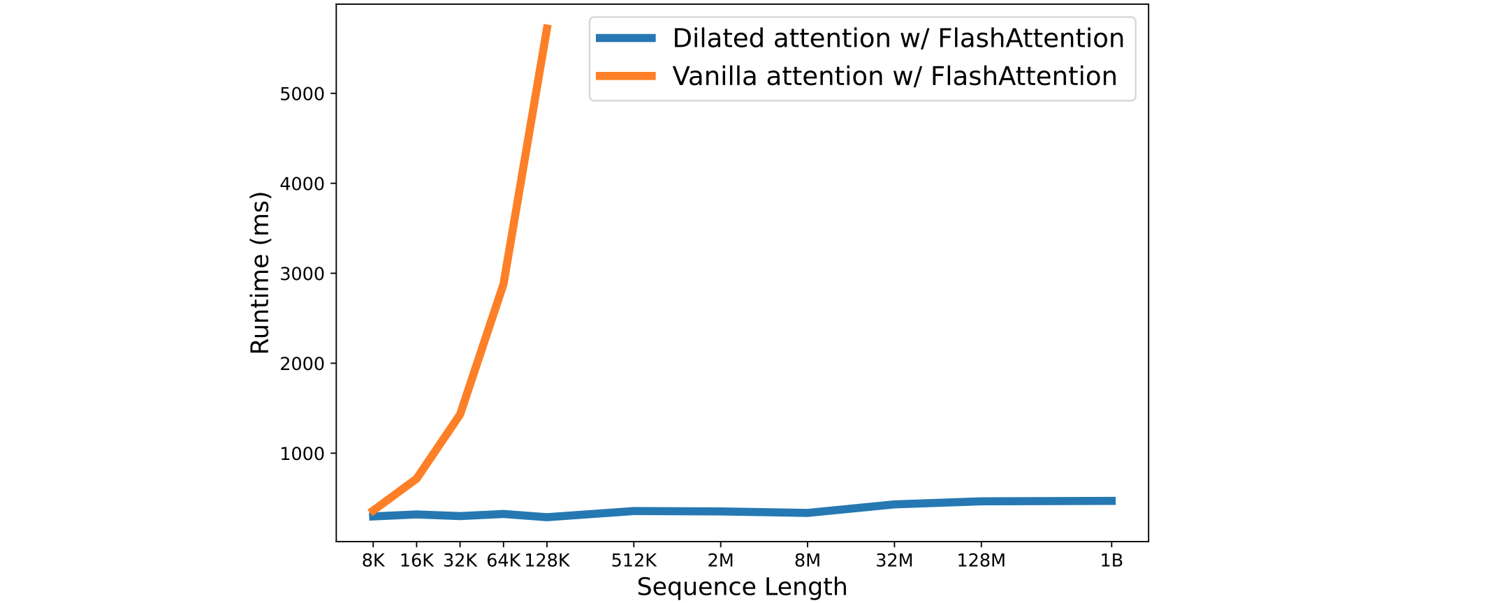
从扩张注意力(Dilated Attention)可以看出,缩放序列长度的延迟几乎是恒定的。因此,可以将序列长度扩展到10亿tokens。而vanilla attention的计算成本与序列长度成二次方关系,导致延迟随着序列长度的增加而迅速增加。此外,vanilla attention没有分布式算法来克服序列长度的限制。结果也显示了LongNet线性复杂度和分布式算法的优越性。
LongNet计算复杂性提高了多少?根据比较,Dilated Attention与普通Attention和Sparse Attention相比,降低了Attention机制的计算复杂度,如下表所示:

上图中:这里的
扩张注意力(Dilated Attention)为什么可以降低计算复杂度?扩张注意力(Dilated Attention)将输入
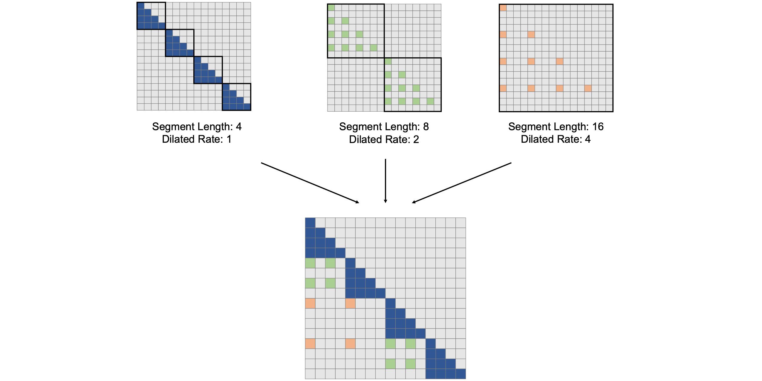
LongNet中使用的扩张注意力的构建块。它由一组注意力模式组成,用于建模长短范围的依赖关系。注意力模式的数量可以根据序列长度进行扩展。如上图所示,通过选取区间

这个经过稀疏化处理的片段

在实际应用中,分段大小Dilated Attention矩阵来降低计算成本。
LongNet分布式训练。Dilated Attention的计算复杂度已经降低到了GPU无法将序列长度扩展到百万量级。因此,提出了用于大规模模型训练的分布式训练算法,如模型并行化、序列处理和流水线处理等。然而,传统方法对于LongNet来说是不够的,尤其是在序列维数较大的情况下。因此,LongNet提出了一种新的分布式算法,该算法可扩展到多个设备而不失通用性。
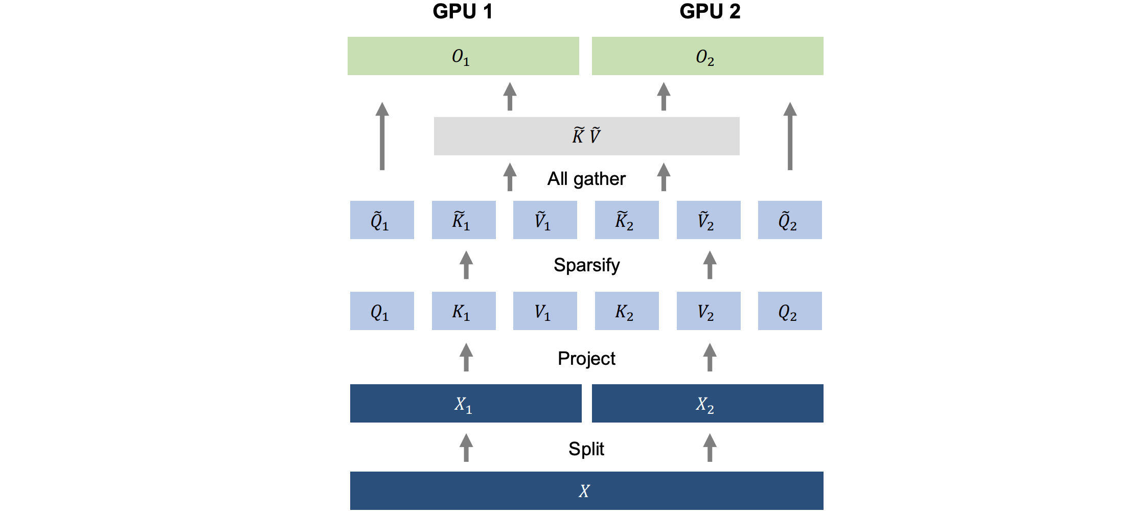
如上图所示,在两台GPU设备上进行LongNet的分布式训练。它通过对序列维度进行分区来并行化训练。随着设备数量的增加,计算和通信成本几乎保持不变。分布式算法流程:
- 输入序列分割:输入序列沿序列维度分割。每个分割后的序列被单独放置在一个设备上。
,两台设备上的查询、键和值也如下所示: 。 - 注意力计算:当
时,即输入段长度( )小于本地设备序列长度( ),则使用 Dilated Attention中的计算方法将其分割;当时,键和值分散在设备上,因此在计算注意力之前,要执行一次全局操作来收集键和值。 。此时,与 Vanilla Attention不同,密钥和值的大小不取决于序列长度,因此通信成本保持不变。 - 计算交叉注意力:使用本地查询和全局键与值计算
Cross Attention:。 - 最终输出:最终的”注意力“输出是不同设备
Kanes输出的合并结果,如下式所示:。
语言建模实验:采用的架构是MAGNETO[WMH+22],使用XPOS[SDP+22]的相对位置编码。它用Dilated Attention取代了标准的Attention。LongNet、Vanilla Transfomer和 Sparse Transfomer进行了比较。在将这些模型的序列长度从2K增加到32K的过程中,似乎对批次大小进行了调整,以保持每个批次的token数不变。此外,由于作者计算环境的限制,他们只对最多32K的token进行了实验。以下是每个语言模型的易错性结果。
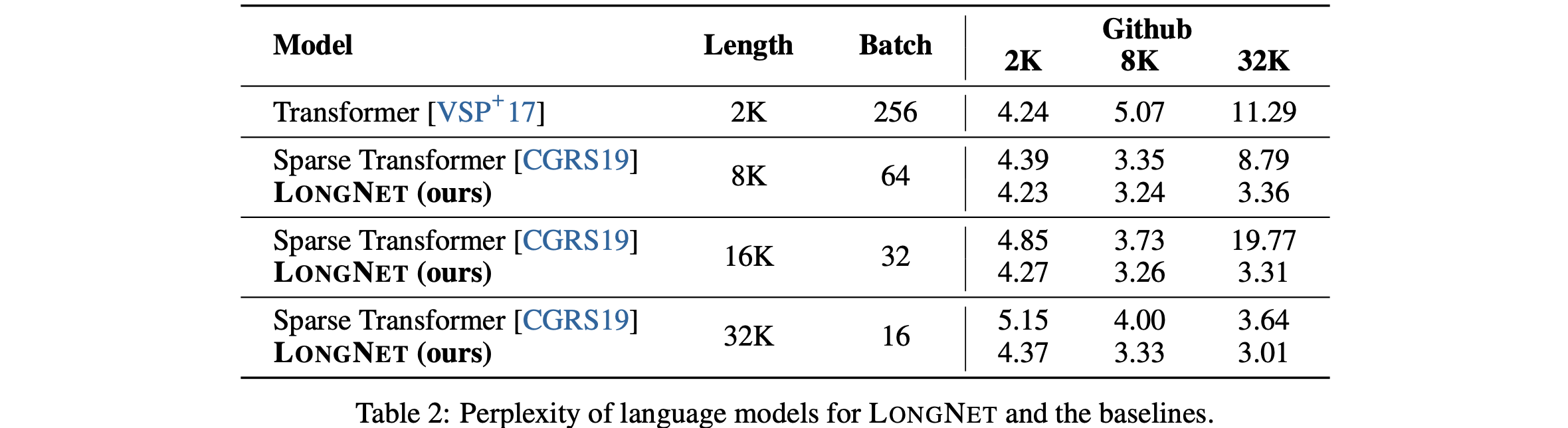
结果证明,在训练过程中增加序列长度可以获得良好的语言模型;在所有情况下,LongNet的表现都优于其他模型,并显示出其有效性。
代码实现
1 | import torch |
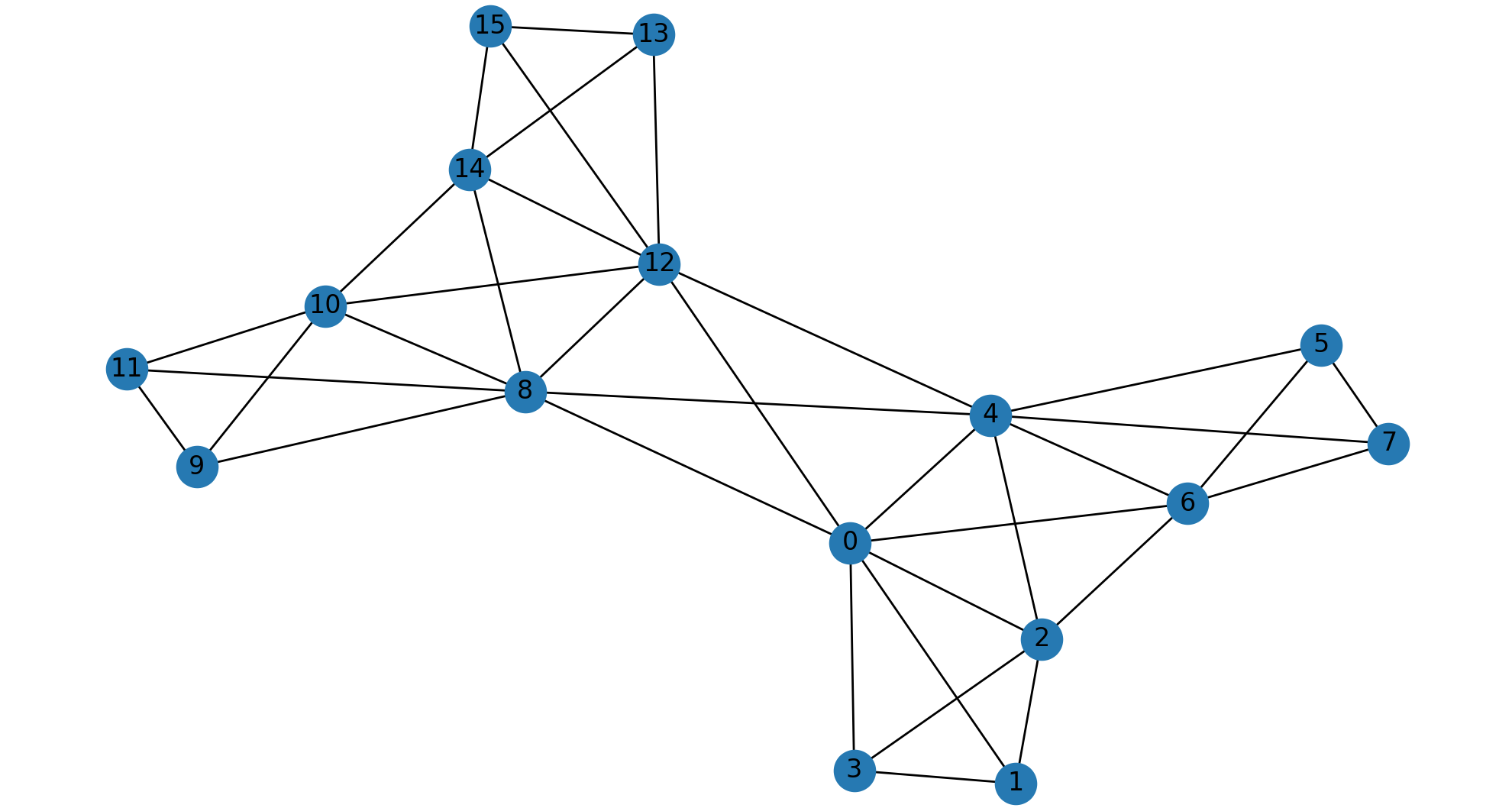
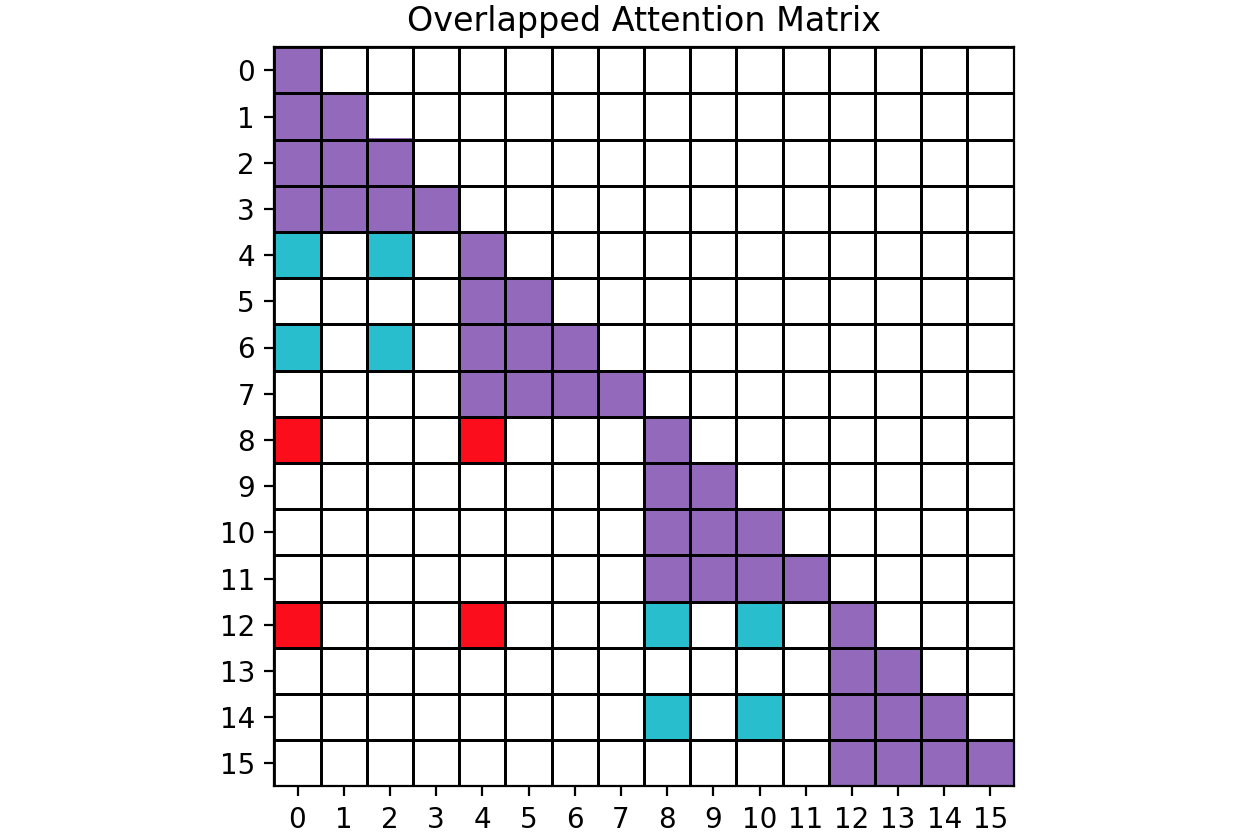
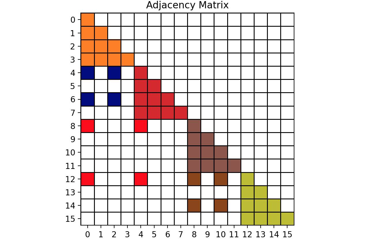
绘制的图如下:重叠注意力矩阵和邻接矩阵:
1 | START_NODE = 5 |
结果输出为:
1 | All nodes are reachable from the node 5 |
1 | import networkx as nx |