对象检测(KerasCV)

对象检测是在给定的图像中识别、分类和定位对象的过程。通常,你的输入是图像,标签是带有可选类标签的边界框。对象检测可以被认为是分类的扩展,但是您必须检测和定位任意数量的类,而不是图像的一个类标签。

上图的数据可能如下所示:

1
2
3
4
5
6
7
8
9
10
11
12
13
14
15
16
17
18
19
20
21
22
import os
from tensorflow import data as tf_data
import tensorflow_datasets as tfds
import keras
import keras_cv
import numpy as np
from keras_cv import bounding_box
import os
from keras_cv import visualization
import tqdm

os.environ["KERAS_BACKEND"] = "jax" # @param ["tensorflow", "jax", "torch"]

image = [height, width, 3]
bounding_boxes = {
"classes": [0], # 0 is an arbitrary class ID representing "cat"
"boxes": [[0.25, 0.4, .15, .1]]
# bounding box is in "rel_xywh" format
# so 0.25 represents the start of the bounding box 25% of
# the way across the image.
# The .15 represents that the width is 15% of the image width.
}

自从You Only Look Once(又名YOLO)问世以来,对象检测主要是通过深度学习来解决的。大多数深度学习架构通过巧妙地将对象检测问题构建为许多小型分类问题和许多回归问题的组合来实现这一点。更具体地说,这是通过在输入图像上生成许多不同形状和大小的锚框并为每个锚框分配一个类标签以及x、y、widthheight偏移来完成的。该模型经过训练可以预测每个框的类标签,以及预测对象的每个框的x、y、widthheight偏移。实际上,输入的图像可能更复杂,并且包含更多对象,在这种情况下,对象检测是通过在输入图像上生成许多不同形状和大小的锚框,并为每个锚框分配一个类标签以及四个数据点来精确定位边界框来完成的,如下图所示:

使用预训练模型执行检测

KerasCV对象检测API中最高级别的APIkeras_cv.models API。此API包括完全预训练的对象检测模型,例如keras_cv.models.YOLOV8Detector。让我们开始构建一个在 pascalvoc数据集上预训练的YOLOV8Detector

1
2
3
4
5
6
7
8
9
10
11
12
13
14
15
16
17
18
19
20
21
22
23
24
25
26
27
28
29
30
31
32
33
34
35
36
37
38
39
40
41
42
43
44
45
46
47
48
49
50
51
52
53
54
55
56
57
58
59
60
61
62
63
64
65
66
67
68
69
70
71
72
73
74
75
76
77
78
79
80
81
82
83
84
85
86
87
88
89
90
91
92
93
94
95
96
97
98
99
100
101
102
103
104
105
106
107
108
109
110
111
112
113
114
115
116
117
118
119
120
121
122
123
124
125
126
127
128
import os
from tensorflow import data as tf_data
import tensorflow_datasets as tfds
import keras
import keras_cv
import numpy as np
from keras_cv import bounding_box
import os
from keras_cv import visualization
import tqdm

os.environ["KERAS_BACKEND"] = "jax" # @param ["tensorflow", "jax", "torch"]

image = keras.utils.load_img(path='dog.jpg')
image = np.array(keras.utils.img_to_array(image))

visualization.plot_image_gallery(
np.array([image]),
value_range=(0, 255),
rows=1,
cols=1,
scale=5,
)

# 要将YOLOV8Detector架构与ResNet50主干结合使用,您需要将图像大小调整为可被64整除的大小。
# 这是为了确保与ResNet中卷积层完成的缩小操作数量兼容。如果调整大小操作扭曲了输入的纵横比,则模型的性能将明显变差。
# 对于我们使用的预训练“yolo_v8_m_pascalvoc”预设,当使用简单的调整大小操作时,pascalvoc/2012 评估集的最终MeanAveragePrecision从0.38下降到0.15。

# 此外,如果您想在分类中那样进行裁剪以保留纵横比,您的模型可能会完全错过一些边界框。
# 因此,在对象检测模型上运行推理时,我们建议使用填充到所需的大小,同时调整最长大小以匹配长宽比。
# KerasCV使调整大小变得容易;只需将pad_to_aspect_ratio=True 传递给keras_cv.layers.Resizing层即可。

inference_resizing = keras_cv.layers.Resizing(
640, 640, pad_to_aspect_ratio=True, bounding_box_format="xywh"
)

# 这可以作为推理预处理管道
image_batch = inference_resizing([image])

# keras_cv.visualization.plot_bounding_box_gallery()支持class_mapping参数来突出显示每个框分配给哪个类。现在让我们组装一个类映射。
class_ids = [
"Aeroplane",
"Bicycle",
"Bird",
"Boat",
"Bottle",
"Bus",
"Car",
"Cat",
"Chair",
"Cow",
"Dining Table",
"Dog",
"Horse",
"Motorbike",
"Person",
"Potted Plant",
"Sheep",
"Sofa",
"Train",
"Tvmonitor",
"Total",
]
class_mapping = dict(zip(range(len(class_ids)), class_ids))
# 为了支持这种简单直观的推理工作流程,KerasCV在YOLOV8Detector类内部执行非最大值抑制。
# 非极大值抑制是一种传统的计算算法,解决模型检测同一对象的多个框的问题。

# 非极大值抑制是一种高度可配置的算法,在大多数情况下,您需要自定义模型的非极大值抑制操作的设置。
# 这可以通过覆盖Prediction_decoder参数来完成。

# 为了展示这个概念,让我们暂时禁用YOLOV8Detector上的非最大抑制。
# 这可以通过写入Prediction_decoder属性来完成。
prediction_decoder = keras_cv.layers.NonMaxSuppression(
bounding_box_format="xywh",
from_logits=True,
iou_threshold=1.0,
confidence_threshold=0.0,
)
pretrained_model = keras_cv.models.YOLOV8Detector.from_preset(
"yolo_v8_m_pascalvoc",
bounding_box_format="xywh",
prediction_decoder=prediction_decoder,
)

y_pred = pretrained_model.predict(image_batch)
visualization.plot_bounding_box_gallery(
image_batch,
value_range=(0, 255),
rows=1,
cols=1,
y_pred=y_pred,
scale=5,
font_scale=0.7,
bounding_box_format="xywh",
class_mapping=class_mapping,
)

# 接下来,让我们的用例重新配置keras_cv.layers.NonMaxSuppression。
# 我们将iou_threshold调整为0.2,将confidence_threshold调整为0.7。

# 提高confidence_threshold将导致模型仅输出具有较高置信度分数的框。
# iou_threshold 控制两个框必须具有的交并集 (IoU) 阈值,以便剪除其中一个框。
prediction_decoder = keras_cv.layers.NonMaxSuppression(
bounding_box_format="xywh",
from_logits=True,
# Decrease the required threshold to make predictions get pruned out
iou_threshold=0.2,
# Tune confidence threshold for predictions to pass NMS
confidence_threshold=0.7,
)
pretrained_model = keras_cv.models.YOLOV8Detector.from_preset(
"yolo_v8_m_pascalvoc",
bounding_box_format="xywh",
prediction_decoder=prediction_decoder,
)

y_pred = pretrained_model.predict(image_batch)
visualization.plot_bounding_box_gallery(
image_batch,
value_range=(0, 255),
rows=1,
cols=1,
y_pred=y_pred,
scale=5,
font_scale=0.7,
bounding_box_format="xywh",
class_mapping=class_mapping,
)

结果输出为:

训练自定义对象检测模型

设置对象检测管道通常具有挑战性,但是,KerasCV正在使其变得简单。我们首先加载PASCAL VOC数据集,可视化数据集确保看起来都是正常的。在执行此操作之前这一步非常重要,因为有时边界框格式会导致出问题。与图像分类类似,我们也可以执行数据增强。我们在tf.data管道内以边界框的方式执行此操作。我们可以看一下结果:

1
2
3
4
5
6
7
8
9
10
11
12
13
14
15
16
17
18
19
20
21
22
23
24
25
26
27
28
29
30
31
32
33
34
35
36
37
38
39
40
41
42
43
44
45
46
47
48
49
50
51
52
53
54
55
56
57
58
59
60
61
62
63
64
65
66
67
68
69
70
71
72
73
74
75
76
77
78
79
80
81
82
83
84
85
86
87
88
89
90
91
92
93
94
95
96
97
98
99
100
101
102
103
104
105
106
107
108
109
110
111
112
113
114
115
116
117
118
119
120
121
122
123
124
125
126
127
128
129
130
131
132
133
134
135
136
137
138
139
140
141
142
143
144
145
146
147
148
149
150
151
152
153
154
155
156
157
158
159
160
161
162
163
164
165
BATCH_SIZE = 4

def visualize_dataset(inputs, value_range, rows, cols, bounding_box_format):
inputs = next(iter(inputs.take(1)))
images, bounding_boxes = inputs["images"], inputs["bounding_boxes"]
visualization.plot_bounding_box_gallery(
images,
value_range=value_range,
rows=rows,
cols=cols,
y_true=bounding_boxes,
scale=5,
font_scale=0.7,
bounding_box_format=bounding_box_format,
class_mapping=class_mapping,
)

def unpackage_raw_tfds_inputs(inputs, bounding_box_format):
image = inputs["image"]
boxes = keras_cv.bounding_box.convert_format(
inputs["objects"]["bbox"],
images=image,
source="rel_yxyx",
target=bounding_box_format,
)
bounding_boxes = {
"classes": inputs["objects"]["label"],
"boxes": boxes,
}
return {"images": image, "bounding_boxes": bounding_boxes}

def load_pascal_voc(split, dataset, bounding_box_format):
ds = tfds.load(dataset, split=split, with_info=False, shuffle_files=True)
ds = ds.map(
lambda x: unpackage_raw_tfds_inputs(x, bounding_box_format=bounding_box_format),
num_parallel_calls=tf_data.AUTOTUNE,
)
return ds

train_ds = load_pascal_voc(split="train", dataset="voc/2007", bounding_box_format="xywh")
eval_ds = load_pascal_voc(split="test", dataset="voc/2007", bounding_box_format="xywh")
train_ds = train_ds.shuffle(BATCH_SIZE * 4)

train_ds = train_ds.ragged_batch(BATCH_SIZE, drop_remainder=True)
eval_ds = eval_ds.ragged_batch(BATCH_SIZE, drop_remainder=True)
visualize_dataset(train_ds, bounding_box_format="xywh", value_range=(0, 255), rows=2, cols=2)

visualize_dataset(
eval_ds,
bounding_box_format="xywh",
value_range=(0, 255),
rows=2,
cols=2,
# If you are not running your experiment on a local machine, you can also
# make `visualize_dataset()` dump the plot to a file using `path`:
# path="eval.png"
)

augmenters = [
keras_cv.layers.RandomFlip(mode="horizontal", bounding_box_format="xywh"),
keras_cv.layers.JitteredResize(
target_size=(640, 640), scale_factor=(0.75, 1.3), bounding_box_format="xywh"
),
]

def create_augmenter_fn(augmenters):
def augmenter_fn(inputs):
for augmenter in augmenters:
inputs = augmenter(inputs)
return inputs

return augmenter_fn

augmenter_fn = create_augmenter_fn(augmenters)
train_ds = train_ds.map(augmenter_fn, num_parallel_calls=tf_data.AUTOTUNE)
visualize_dataset(train_ds, bounding_box_format="xywh", value_range=(0, 255), rows=2, cols=2)

inference_resizing = keras_cv.layers.Resizing(640, 640, bounding_box_format="xywh", pad_to_aspect_ratio=True)
eval_ds = eval_ds.map(inference_resizing, num_parallel_calls=tf_data.AUTOTUNE)

def dict_to_tuple(inputs):
return inputs["images"], bounding_box.to_dense(inputs["bounding_boxes"], max_boxes=32)

train_ds = train_ds.map(dict_to_tuple, num_parallel_calls=tf_data.AUTOTUNE)
eval_ds = eval_ds.map(dict_to_tuple, num_parallel_calls=tf_data.AUTOTUNE)

train_ds = train_ds.prefetch(tf_data.AUTOTUNE)
eval_ds = eval_ds.prefetch(tf_data.AUTOTUNE)

# 定义SGD优化器
base_lr = 0.005
# including a global_clipnorm is extremely important in object detection tasks
optimizer = keras.optimizers.SGD(
learning_rate=base_lr, momentum=0.9, global_clipnorm=10.0
)

pretrained_model.compile(
classification_loss="binary_crossentropy",
box_loss="ciou",
)

# 最流行的对象检测指标是COCO指标,它与MSCOCO数据集一起发布。
# KerasCV在 keras_cv.callbacks.PyCOCOCallback下提供了一套易于使用的COCO指标。
# 请注意,我们使用Keras回调而不是Keras指标来计算COCO指标。
# 这是因为计算COCO指标需要将模型对整个评估数据集的所有预测立即存储在内存中,这在训练期间是不切实际的。
coco_metrics_callback = keras_cv.callbacks.PyCOCOCallback(eval_ds.take(20), bounding_box_format="xywh")

# 模型创建
# 接下来,我们使用KerasCV API构建一个未经训练的YOLOV8Detector模型。
model = keras_cv.models.YOLOV8Detector.from_preset(
"resnet50_imagenet",
# For more info on supported bounding box formats, visit
bounding_box_format="xywh",
num_classes=20,
)

# 剩下要做的就是训练我们的模型。KerasCV对象检测模型遵循标准Keras工作流程,利用compile()和fit()。让我们编译模型:
model.compile(
classification_loss="binary_crossentropy",
box_loss="ciou",
optimizer=optimizer,
)

# 如果您想完全训练模型,请输入train_ds.take(20):
model.fit(
train_ds.take(20),
# Run for 10-35~ epochs to achieve good scores.
epochs=1,
callbacks=[coco_metrics_callback],
)

# model.predict(images)返回边界框张量。默认情况下,YOLOV8Detector.predict()将为您执行非极大值抑制操作。
model = keras_cv.models.YOLOV8Detector.from_preset("yolo_v8_m_pascalvoc", bounding_box_format="xywh")

# 接下来,我们构建一个具有更大批次的数据集:
visualization_ds = eval_ds.unbatch()
visualization_ds = visualization_ds.ragged_batch(16)
visualization_ds = visualization_ds.shuffle(8)

def visualize_detections(model, dataset, bounding_box_format):
images, y_true = next(iter(dataset.take(1)))
y_pred = model.predict(images)
visualization.plot_bounding_box_gallery(
images,
value_range=(0, 255),
bounding_box_format=bounding_box_format,
y_true=y_true,
y_pred=y_pred,
scale=4,
rows=2,
cols=2,
show=True,
font_scale=0.7,
class_mapping=class_mapping,
)

# 您可能需要配置NonMaxSuppression操作以获得更好的结果。
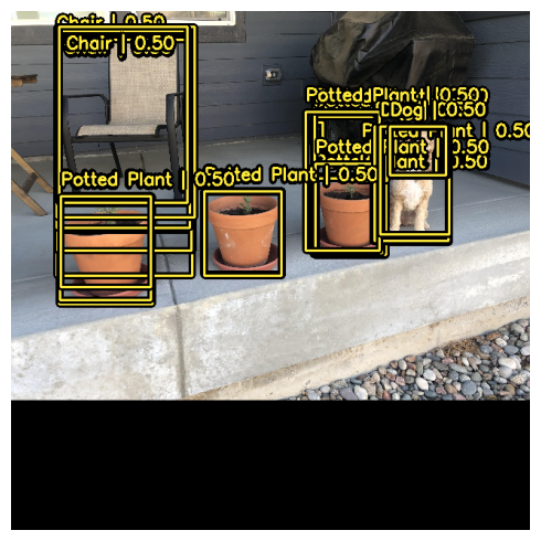
model.prediction_decoder = keras_cv.layers.NonMaxSuppression(
bounding_box_format="xywh",
from_logits=True,
iou_threshold=0.5,
confidence_threshold=0.75,
)

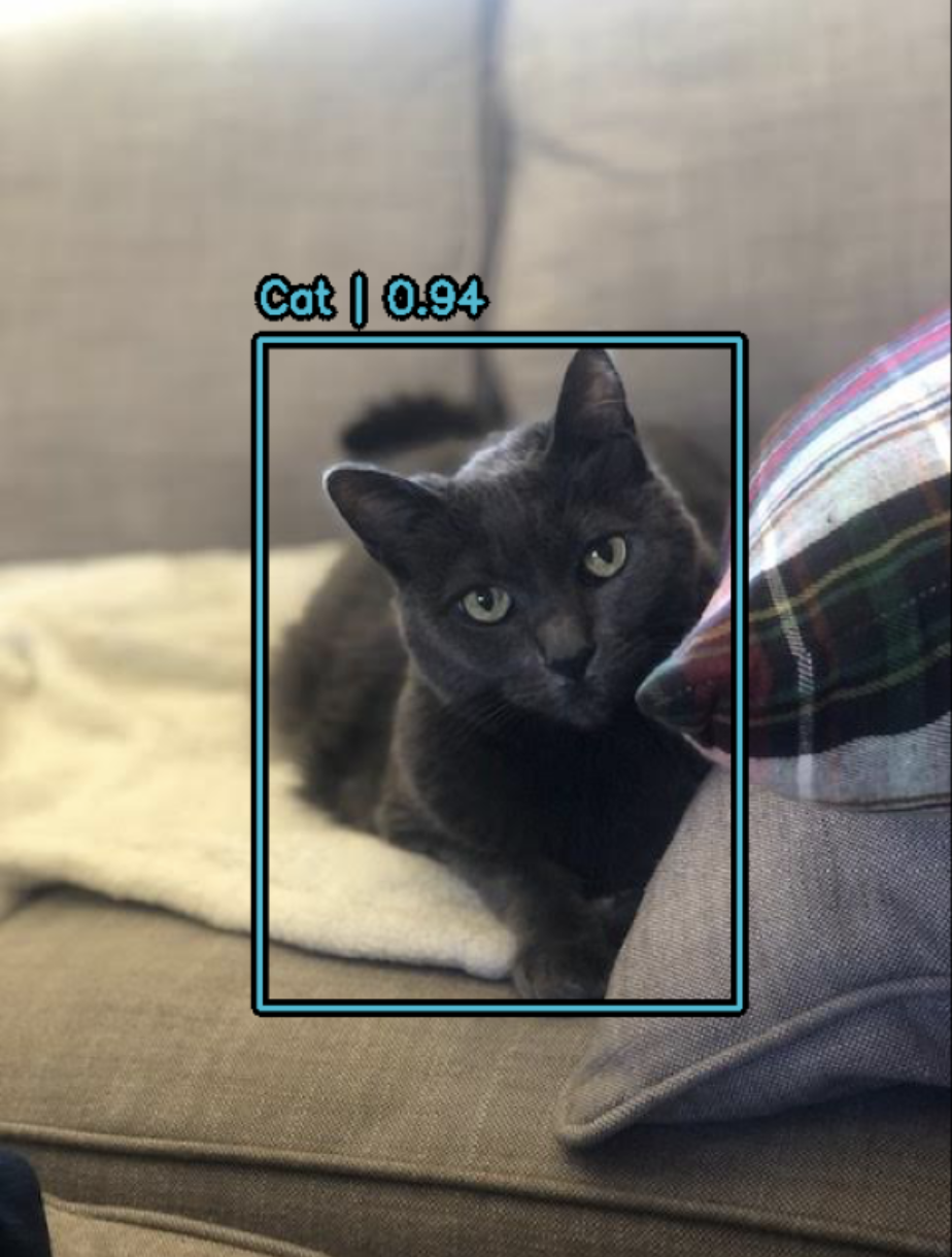
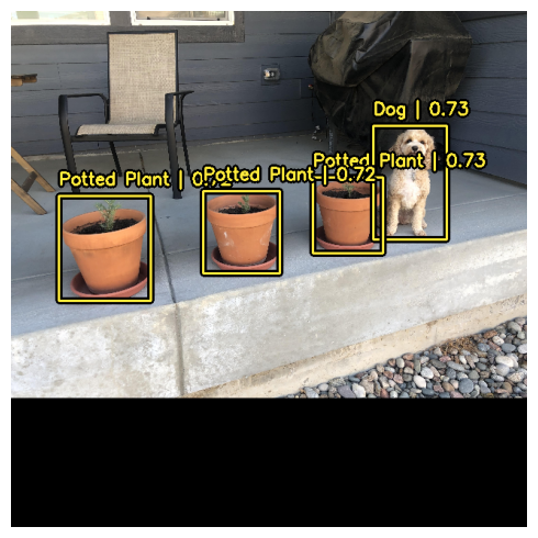
visualize_detections(model, dataset=visualization_ds, bounding_box_format="xywh")

KerasCV可以轻松构建最先进的对象检测管道。我们首先使用KerasCV边界框规范编写数据加载器。接下来,我们使用KerasCV预处理层在不到50行的代码中组装了一个生产级数据增强管道。KerasCV对象检测组件可以独立使用,也可以深度集成。KerasCV使创作生产级边界框增强、模型训练、可视化和指标评估变得更容易。