您将获得每日历史销售数据。任务是预测测试集每个商店销售的产品总量。请注意,商店和产品列表每个月都会略有变化。创建一个可以处理此类情况的强大模型是挑战的一部分。
包和加载数据 1 2 3 4 5 6 7 8 9 10 11 12 13 14 15 16 17 18 19 20 21 22 23 24 25 26 27 28 29 30 31 32 33 34 35 36 37 38 39 40 41 42 43 44 45 46 import warningsimport numpy as npimport pandas as pdimport matplotlib.pyplot as pltfrom keras import optimizersfrom keras.utils import plot_modelfrom keras.models import Sequential, Modelfrom keras.layers.convolutional import Conv1D, MaxPooling1Dfrom keras.layers import Dense, LSTM, RepeatVector, TimeDistributed, Flattenfrom sklearn.metrics import mean_squared_errorfrom sklearn.model_selection import train_test_splitimport plotly.plotly as pyimport plotly.graph_objs as gofrom plotly.offline import init_notebook_mode, iplotwarnings.filterwarnings("ignore" ) from tensorflow import set_random_seedfrom numpy.random import seedset_random_seed(1 ) seed(1 ) train = pd.read_csv('../input/demand-forecasting-kernels-only/train.csv' , parse_dates=['date' ]) test = pd.read_csv('../input/demand-forecasting-kernels-only/test.csv' , parse_dates=['date' ]) train.describe() train.head()
训练数据集的时间段:
1
2
3
4
5
print ('Min date from train set: %s' % train['date' ].min ().date())print ('Max date from train set: %s' % train['date' ].max ().date())
让我们找出训练集的最后一天与测试集的最后一天之间的时间差距是多少,这将是滞后(需要预测的天数)。
1
2
3
4
5
6
7
8
lag_size = (test['date' ].max ().date() - train['date' ].max ().date()).days print ('Max date from train set: %s' % train['date' ].max ().date())print ('Max date from test set: %s' % test['date' ].max ().date())print ('Forecast lag size' , lag_size)Max date from train set : 2017 -12 -31 Max date from test set : 2018 -03-31 Forecast lag size 90
使用ploty进行时间序列可视化 首先探索时间序列数据:
1 2 3 4 5 6 7 8 9 10 11 12 13 14 15 16 17 18 19 20 21 22 23 24 25 26 27 28 29 30 daily_sales = train.groupby('date' , as_index=False )['sales' ].sum () store_daily_sales = train.groupby(['store' , 'date' ], as_index=False )['sales' ].sum () item_daily_sales = train.groupby(['item' , 'date' ], as_index=False )['sales' ].sum () daily_sales_sc = go.Scatter(x=daily_sales['date' ], y=daily_sales['sales' ]) layout = go.Layout(title='Daily sales' , xaxis=dict (title='Date' ), yaxis=dict (title='Sales' )) fig = go.Figure(data=[daily_sales_sc], layout=layout) iplot(fig) store_daily_sales_sc = [] for store in store_daily_sales['store' ].unique(): current_store_daily_sales = store_daily_sales[(store_daily_sales['store' ] == store)] store_daily_sales_sc.append(go.Scatter(x=current_store_daily_sales['date' ], y=current_store_daily_sales['sales' ], name=('Store %s' % store))) layout = go.Layout(title='Store daily sales' , xaxis=dict (title='Date' ), yaxis=dict (title='Sales' )) fig = go.Figure(data=store_daily_sales_sc, layout=layout) iplot(fig) item_daily_sales_sc = [] for item in item_daily_sales['item' ].unique(): current_item_daily_sales = item_daily_sales[(item_daily_sales['item' ] == item)] item_daily_sales_sc.append(go.Scatter(x=current_item_daily_sales['date' ], y=current_item_daily_sales['sales' ], name=('Item %s' % item))) layout = go.Layout(title='Item daily sales' , xaxis=dict (title='Date' ), yaxis=dict (title='Sales' )) fig = go.Figure(data=item_daily_sales_sc, layout=layout) iplot(fig)
子样本训练集仅获取最后一年的数据并减少训练时间,重新排列数据集,以便我们可以应用移位方法。
1
2
3
4
5
6
7
8
9
10
11
12
train = train[(train['date' ] >= '2017-01-01' )] train_gp = train.sort_values('date' ).groupby(['item' , 'store' , 'date' ], as_index=False ) train_gp = train_gp.agg({'sales' :['mean' ]}) train_gp.columns = ['item' , 'store' , 'date' , 'sales' ] train_gp.head()
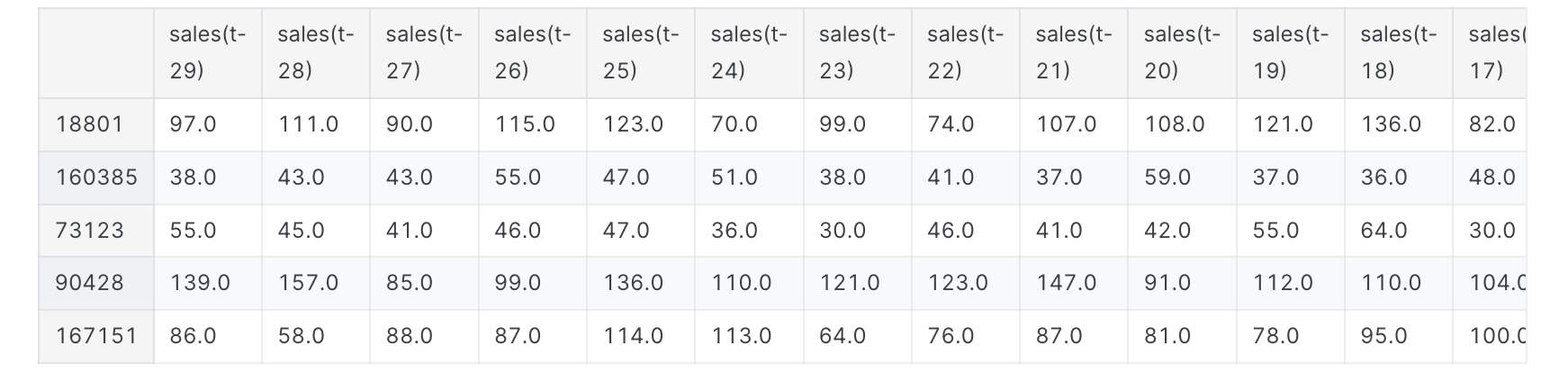
如何将时间序列数据集转换为监督学习问题? 将数据转化为时间序列问题,我们将使用当前时间步长和最近29个时间步长来预测未来90天
1
2
3
4
5
6
7
8
9
10
11
12
13
14
15
16
17
18
19
20
21
22
23
24
def series_to_supervised (data, window=1 , lag=1 , dropnan=True ): cols, names = list (), list () for i in range (window, 0 , -1 ): cols.append(data.shift(i)) names += [('%s(t-%d)' % (col, i)) for col in data.columns] cols.append(data) names += [('%s(t)' % (col)) for col in data.columns] cols.append(data.shift(-lag)) names += [('%s(t+%d)' % (col, lag)) for col in data.columns] agg = pd.concat(cols, axis=1 ) agg.columns = names if dropnan: agg.dropna(inplace=True ) return agg window = 29 lag = lag_size series = series_to_supervised(train_gp.drop('date' , axis=1 ), window=window, lag=lag) series.head()
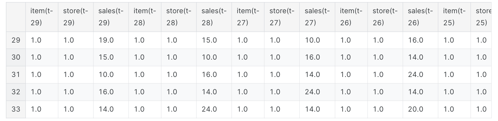
删除具有与移位列不同的项目或存储值的行,删除不需要的列。训练/验证分割。
1
2
3
4
5
6
7
8
9
10
11
12
13
14
15
16
17
18
19
20
21
22
23
last_item = 'item(t-%d)' % window last_store = 'store(t-%d)' % window series = series[(series['store(t)' ] == series[last_store])] series = series[(series['item(t)' ] == series[last_item])] columns_to_drop = [('%s(t+%d)' % (col, lag)) for col in ['item' , 'store' ]] for i in range (window, 0 , -1 ): columns_to_drop += [('%s(t-%d)' % (col, i)) for col in ['item' , 'store' ]] series.drop(columns_to_drop, axis=1 , inplace=True ) series.drop(['item(t)' , 'store(t)' ], axis=1 , inplace=True ) labels_col = 'sales(t+%d)' % lag_size labels = series[labels_col] series = series.drop(labels_col, axis=1 ) X_train, X_valid, Y_train, Y_valid = train_test_split(series, labels.values, test_size=0.4 , random_state=0 ) print ('Train set shape' , X_train.shape)print ('Validation set shape' , X_valid.shape)X_train.head()
如何为单变量时间序列预测问题开发多层感知器模型 用于时间序列预测的MLP:
首先,我们将使用多层感知器模型或MLP模型,这里我们的模型将具有等于窗口大小的输入特征。
MLP模型的问题是,模型不将输入视为排序数据,因此对于模型来说,它只是接收输入,而不将它们视为排序数据,这可能是一个问题,因为模型不会查看具有序列模式的数据。输入形状[samples, timesteps]。
1
2
3
4
5
6
7
8
9
10
11
12
13
14
15
16
17
18
19
20
21
22
23
24
25
epochs = 40 batch = 256 lr = 0.0003 adam = optimizers.Adam(lr) model_mlp = Sequential() model_mlp.add(Dense(100 , activation='relu' , input_dim=X_train.shape[1 ])) model_mlp.add(Dense(1 )) model_mlp.compile (loss='mse' , optimizer=adam) model_mlp.summary() mlp_history = model_mlp.fit(X_train.values, Y_train, validation_data=(X_valid.values, Y_valid), epochs=epochs, verbose=2 )
如何针对单变量时间序列预测问题开发卷积神经网络模型 用于时间序列预测的CNN:
对于CNN模型,我们将使用一个卷积隐藏层,后跟一个最大池化层。然后,滤波器图在由密集层解释并输出预测之前被展平。
卷积层应该能够识别时间步之间的模式。
输入形状[samples, timesteps, features]。
数据预处理:
从[samples, timesteps]重塑为 [samples, timesteps, features]。
同样的重塑数据将用于CNN和LSTM模型。
1
2
3
4
5
6
7
8
9
10
11
12
13
14
15
16
17
18
19
20
21
22
23
24
25
26
27
28
29
30
31
32
33
34
35
36
37
X_train_series = X_train.values.reshape((X_train.shape[0 ], X_train.shape[1 ], 1 )) X_valid_series = X_valid.values.reshape((X_valid.shape[0 ], X_valid.shape[1 ], 1 )) print ('Train set shape' , X_train_series.shape)print ('Validation set shape' , X_valid_series.shape)model_cnn = Sequential() model_cnn.add(Conv1D(filters=64 , kernel_size=2 , activation='relu' , input_shape=(X_train_series.shape[1 ], X_train_series.shape[2 ]))) model_cnn.add(MaxPooling1D(pool_size=2 )) model_cnn.add(Flatten()) model_cnn.add(Dense(50 , activation='relu' )) model_cnn.add(Dense(1 )) model_cnn.compile (loss='mse' , optimizer=adam) model_cnn.summary() cnn_history = model_cnn.fit(X_train_series, Y_train, validation_data=(X_valid_series, Y_valid), epochs=epochs, verbose=2 )
如何针对单变量时间序列预测问题开发长短期记忆网络模型 用于时间序列预测的LSTM:
LSTM模型实际上将输入数据视为序列,因此它能够比其他数据更好地从序列数据中学习模式,尤其是长序列中的模式。输入形状[samples, timesteps, features]。
1
2
3
4
5
6
7
8
9
10
11
12
13
14
15
16
17
18
19
20
model_lstm = Sequential() model_lstm.add(LSTM(50 , activation='relu' , input_shape=(X_train_series.shape[1 ], X_train_series.shape[2 ]))) model_lstm.add(Dense(1 )) model_lstm.compile (loss='mse' , optimizer=adam) model_lstm.summary() lstm_history = model_lstm.fit(X_train_series, Y_train, validation_data=(X_valid_series, Y_valid), epochs=epochs, verbose=2 )
如何针对单变量时间序列预测问题开发混合CNN-LSTM模型 用于时间序列预测的CNN-LSTM:
输入形状[samples, subsequences, timesteps, features]
模型解释:
“这个模型的好处是,该模型可以支持非常长的输入序列,这些序列可以被CNN模型读取为块或子序列,然后由LSTM模型拼凑在一起。”
“当使用混合CNN-LSTM模型时,我们将把每个样本进一步划分为更多的子序列。CNN模型将解释每个子序列,LSTM将把子序列的解释拼凑在一起。因此,我们将每个样本划分为2个子序列,每个子序列2次。”
“CNN将被定义为每个子序列有2个时间步,具有一个特征。然后整个CNN模型被包装在TimeDistributed包装层中,以便它可以应用于样本中的每个子序列。然后由LSTM层解释结果。模型输出预测。”
数据预处理:
将[samples, timesteps, features]重塑为[samples, subsequences, timesteps, features]。
1
2
3
4
5
6
7
8
9
10
11
12
13
14
15
16
17
18
19
20
21
subsequences = 2 timesteps = X_train_series.shape[1 ]//subsequences X_train_series_sub = X_train_series.reshape((X_train_series.shape[0 ], subsequences, timesteps, 1 )) X_valid_series_sub = X_valid_series.reshape((X_valid_series.shape[0 ], subsequences, timesteps, 1 )) print ('Train set shape' , X_train_series_sub.shape)print ('Validation set shape' , X_valid_series_sub.shape)model_cnn_lstm = Sequential() model_cnn_lstm.add(TimeDistributed(Conv1D(filters=64 , kernel_size=1 , activation='relu' ), input_shape=(None , X_train_series_sub.shape[2 ], X_train_series_sub.shape[3 ]))) model_cnn_lstm.add(TimeDistributed(MaxPooling1D(pool_size=2 ))) model_cnn_lstm.add(TimeDistributed(Flatten())) model_cnn_lstm.add(LSTM(50 , activation='relu' )) model_cnn_lstm.add(Dense(1 )) model_cnn_lstm.compile (loss='mse' , optimizer=adam) cnn_lstm_history = model_cnn_lstm.fit(X_train_series_sub, Y_train, validation_data=(X_valid_series_sub, Y_valid), epochs=epochs, verbose=2 )
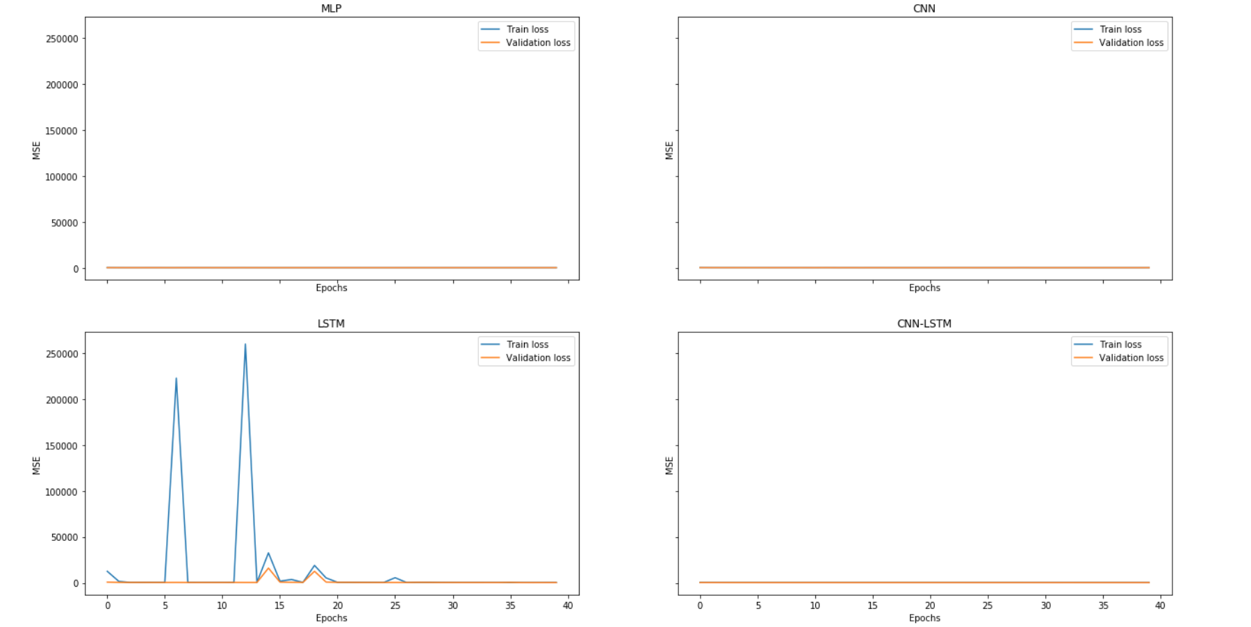
模型比较 1 2 3 4 5 6 7 8 9 10 11 12 13 14 15 16 17 18 19 20 21 22 23 24 25 26 27 28 29 30 31 32 33 fig, axes = plt.subplots(2 , 2 , sharex=True , sharey=True ,figsize=(22 ,12 )) ax1, ax2 = axes[0 ] ax3, ax4 = axes[1 ] ax1.plot(mlp_history.history['loss' ], label='Train loss' ) ax1.plot(mlp_history.history['val_loss' ], label='Validation loss' ) ax1.legend(loc='best' ) ax1.set_title('MLP' ) ax1.set_xlabel('Epochs' ) ax1.set_ylabel('MSE' ) ax2.plot(cnn_history.history['loss' ], label='Train loss' ) ax2.plot(cnn_history.history['val_loss' ], label='Validation loss' ) ax2.legend(loc='best' ) ax2.set_title('CNN' ) ax2.set_xlabel('Epochs' ) ax2.set_ylabel('MSE' ) ax3.plot(lstm_history.history['loss' ], label='Train loss' ) ax3.plot(lstm_history.history['val_loss' ], label='Validation loss' ) ax3.legend(loc='best' ) ax3.set_title('LSTM' ) ax3.set_xlabel('Epochs' ) ax3.set_ylabel('MSE' ) ax4.plot(cnn_lstm_history.history['loss' ], label='Train loss' ) ax4.plot(cnn_lstm_history.history['val_loss' ], label='Validation loss' ) ax4.legend(loc='best' ) ax4.set_title('CNN-LSTM' ) ax4.set_xlabel('Epochs' ) ax4.set_ylabel('MSE' ) plt.show()
1 2 3 4 5 6 7 8 9 10 11 12 13 14 15 16 17 18 19 20 21 22 23 24 25 26 27 28 29 30 31 32 33 34 35 mlp_train_pred = model_mlp.predict(X_train.values) mlp_valid_pred = model_mlp.predict(X_valid.values) print ('Train rmse:' , np.sqrt(mean_squared_error(Y_train, mlp_train_pred)))print ('Validation rmse:' , np.sqrt(mean_squared_error(Y_valid, mlp_valid_pred)))cnn_train_pred = model_cnn.predict(X_train_series) cnn_valid_pred = model_cnn.predict(X_valid_series) print ('Train rmse:' , np.sqrt(mean_squared_error(Y_train, cnn_train_pred)))print ('Validation rmse:' , np.sqrt(mean_squared_error(Y_valid, cnn_valid_pred)))lstm_train_pred = model_lstm.predict(X_train_series) lstm_valid_pred = model_cnn.predict(X_valid_series) print ('Train rmse:' , np.sqrt(mean_squared_error(Y_train, lstm_train_pred)))print ('Validation rmse:' , np.sqrt(mean_squared_error(Y_valid, lstm_valid_pred)))cnn_lstm_train_pred = model_cnn_lstm.predict(X_train_series_sub) cnn_lstm_valid_pred = model_cnn_lstm.predict(X_valid_series_sub) print ('Train rmse:' , np.sqrt(mean_squared_error(Y_train, cnn_lstm_train_pred)))print ('Validation rmse:' , np.sqrt(mean_squared_error(Y_valid, cnn_lstm_valid_pred)))Train rmse: 19.204481417234568 Validation rmse: 19.17420051024767
结论 在这里你可以看到一些解决时间序列问题的方法,如何开发以及它们之间的区别,这并不意味着有很好的性能,所以如果你想要更好的结果,你可以尝试几种不同的超参数(hyper-parameters),特别是窗口大小和网络拓扑 。