情绪检测(TensorFlow)

该数据集包含35,68548x48像素灰度图像的示例,分为训练数据集和测试数据集。根据面部表情中显示的情绪对图像进行分类(快乐、中性、悲伤、愤怒、惊讶、厌恶、恐惧)。

包和配置

1
2
3
4
5
6
7
8
9
10
11
12
13
14
15
16
17
18
19
20
21
22
23
24
25
26
27
28
29
30
31
32
# facial expressions:(happiness, neutral, sadness, anger, surprise, disgust, fear)

import pandas as pd
import numpy as np
import matplotlib.pyplot as plt
import seaborn as sns
import plotly.express as px
import tensorflow as tf
from tensorflow.keras.preprocessing.image import ImageDataGenerator
from tensorflow.keras.utils import to_categorical
from sklearn.metrics import confusion_matrix , classification_report
from sklearn.preprocessing import LabelBinarizer
from sklearn.metrics import roc_curve, auc, roc_auc_score
from IPython.display import clear_output
import warnings

warnings.filterwarnings('ignore')
train_dir = "../input/emotion-detection-fer/train"
test_dir = "../input/emotion-detection-fer/test"

SEED = 12
IMG_HEIGHT = 48
IMG_WIDTH = 48
BATCH_SIZE = 64
EPOCHS = 30
FINE_TUNING_EPOCHS = 20
LR = 0.01
NUM_CLASSES = 7
EARLY_STOPPING_CRITERIA=3
CLASS_LABELS = ['Anger', 'Disgust', 'Fear', 'Happy', 'Neutral', 'Sadness', "Surprise"]
CLASS_LABELS_EMOJIS = ["👿", "🤢" , "😱" , "😊" , "😐 ", "😔" , "😲" ]

数据加载和预处理

1
2
3
4
5
6
7
8
9
10
11
12
13
14
15
16
17
18
19
20
21
22
23
24
25
26
27
28
29
30
31
32
33
34
35
36
37
38
39
40
41
42
43
44
45
46
47
48
49
50
51
52
53
54
55
56
57
58
59
60
61
62
63
64
65
66
67
68
69
70
71
72
73
74
75
76
77
78
79
80
81
82
83
84
85
86
87
88
89
90
91
92
93
94
95
96
97
98
99
100
101
102
103
104
105
106
107
108
109
110
111
112
preprocess_fun = tf.keras.applications.densenet.preprocess_input

train_datagen = ImageDataGenerator(horizontal_flip=True,
width_shift_range=0.1,
height_shift_range=0.05,
rescale = 1./255,
validation_split = 0.2,
preprocessing_function=preprocess_fun
)
test_datagen = ImageDataGenerator(rescale = 1./255,
validation_split = 0.2,
preprocessing_function=preprocess_fun)

train_generator = train_datagen.flow_from_directory(directory = train_dir,
target_size = (IMG_HEIGHT ,IMG_WIDTH),
batch_size = BATCH_SIZE,
shuffle = True ,
color_mode = "rgb",
class_mode = "categorical",
subset = "training",
seed = 12
)

validation_generator = test_datagen.flow_from_directory(directory = train_dir,
target_size = (IMG_HEIGHT ,IMG_WIDTH),
batch_size = BATCH_SIZE,
shuffle = True ,
color_mode = "rgb",
class_mode = "categorical",
subset = "validation",
seed = 12
)

test_generator = test_datagen.flow_from_directory(directory = test_dir,
target_size = (IMG_HEIGHT ,IMG_WIDTH),
batch_size = BATCH_SIZE,
shuffle = False ,
color_mode = "rgb",
class_mode = "categorical",
seed = 12
)

# Found 22968 images belonging to 7 classes.
# Found 5741 images belonging to 7 classes.
# Found 7178 images belonging to 7 classes.

# Helper Functions
def display_one_image(image, title, subplot, color):
plt.subplot(subplot)
plt.axis('off')
plt.imshow(image)
plt.title(title, fontsize=16)

def display_nine_images(images, titles, title_colors=None):
subplot = 331
plt.figure(figsize=(13,13))
for i in range(9):
color = 'black' if title_colors is None else title_colors[i]
display_one_image(images[i], titles[i], 331+i, color)
plt.tight_layout()
plt.subplots_adjust(wspace=0.1, hspace=0.1)
plt.show()

def image_title(label, prediction):
# Both prediction (probabilities) and label (one-hot) are arrays with one item per class.
class_idx = np.argmax(label, axis=-1)
prediction_idx = np.argmax(prediction, axis=-1)
if class_idx == prediction_idx:
return f'{CLASS_LABELS[prediction_idx]} [correct]', 'black'
else:
return f'{CLASS_LABELS[prediction_idx]} [incorrect, should be {CLASS_LABELS[class_idx]}]', 'red'

def get_titles(images, labels, model):
predictions = model.predict(images)
titles, colors = [], []
for label, prediction in zip(classes, predictions):
title, color = image_title(label, prediction)
titles.append(title)
colors.append(color)
return titles, colors

img_datagen = ImageDataGenerator(rescale = 1./255)
img_generator = img_datagen.flow_from_directory(directory = train_dir,
target_size = (IMG_HEIGHT ,IMG_WIDTH),
batch_size = BATCH_SIZE,
shuffle = True ,
color_mode = "rgb",
class_mode = "categorical",
seed = 12
)
clear_output()
# 不同情绪的图像
images, classes = next(img_generator)
class_idxs = np.argmax(classes, axis=-1)
labels = [CLASS_LABELS[idx] for idx in class_idxs]
display_nine_images(images, labels)

# 不同情绪之间的数据分布(计数)
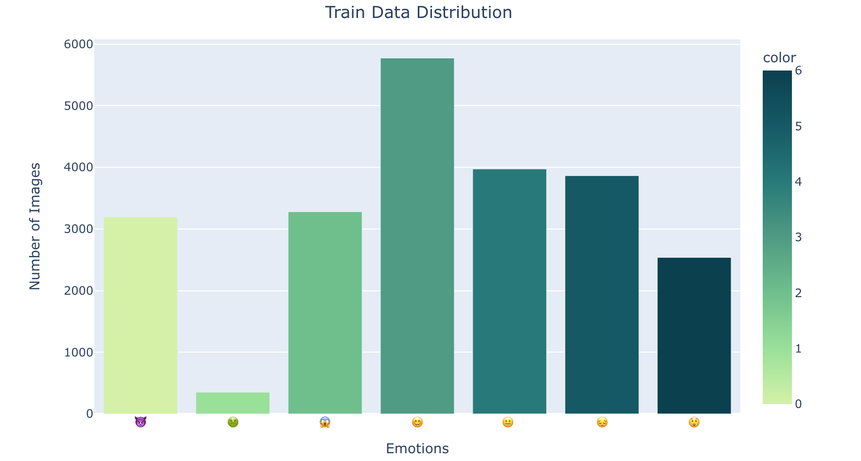
fig = px.bar(x = CLASS_LABELS_EMOJIS,
y = [list(train_generator.classes).count(i) for i in np.unique(train_generator.classes)] ,
color = np.unique(train_generator.classes) ,
color_continuous_scale="Emrld")
fig.update_xaxes(title="Emotions")
fig.update_yaxes(title = "Number of Images")
fig.update_layout(showlegend = True,
title = {
'text': 'Train Data Distribution ',
'y':0.95,
'x':0.5,
'xanchor': 'center',
'yanchor': 'top'})
fig.show()
1
2
3
4
5
6
7
8
9
10
11
12
13
14
15
16
17
18
19
20
21
22
23
24
25
26
27
28
29
30
31
32
33
34
35
36
37
38
39
40
41
42
43
44
45
# DenseNet169 迁移学习

def feature_extractor(inputs):
feature_extractor = tf.keras.applications.DenseNet169(input_shape=(IMG_HEIGHT,IMG_WIDTH, 3),
include_top=False,
weights="imagenet")(inputs)

return feature_extractor

def classifier(inputs):
x = tf.keras.layers.GlobalAveragePooling2D()(inputs)
x = tf.keras.layers.Dense(256, activation="relu", kernel_regularizer = tf.keras.regularizers.l2(0.01))(x)
x = tf.keras.layers.Dropout(0.3)(x)
x = tf.keras.layers.Dense(1024, activation="relu", kernel_regularizer = tf.keras.regularizers.l2(0.01))(x)
x = tf.keras.layers.Dropout(0.5)(x)
x = tf.keras.layers.Dense(512, activation="relu", kernel_regularizer = tf.keras.regularizers.l2(0.01))(x)
x = tf.keras.layers.Dropout(0.5) (x)
x = tf.keras.layers.Dense(NUM_CLASSES, activation="softmax", name="classification")(x)

return x

def final_model(inputs):
densenet_feature_extractor = feature_extractor(inputs)
classification_output = classifier(densenet_feature_extractor)

return classification_output

def define_compile_model():

inputs = tf.keras.layers.Input(shape=(IMG_HEIGHT ,IMG_WIDTH,3))
classification_output = final_model(inputs)
model = tf.keras.Model(inputs=inputs, outputs = classification_output)

model.compile(optimizer=tf.keras.optimizers.SGD(0.1), loss='categorical_crossentropy',metrics = ['accuracy'])

return model


model = define_compile_model()
clear_output()

# Feezing the feature extraction layers
model.layers[1].trainable = False

model.summary()

结果输出为:

1
2
3
4
5
6
7
8
9
10
11
12
13
14
15
16
17
18
19
20
21
22
23
24
25
26
27
28
Model: "model"
_________________________________________________________________
Layer (type) Output Shape Param #
=================================================================
input_1 (InputLayer) [(None, 48, 48, 3)] 0
_________________________________________________________________
densenet169 (Functional) (None, 1, 1, 1664) 12642880
_________________________________________________________________
global_average_pooling2d (Gl (None, 1664) 0
_________________________________________________________________
dense (Dense) (None, 256) 426240
_________________________________________________________________
dropout (Dropout) (None, 256) 0
_________________________________________________________________
dense_1 (Dense) (None, 1024) 263168
_________________________________________________________________
dropout_1 (Dropout) (None, 1024) 0
_________________________________________________________________
dense_2 (Dense) (None, 512) 524800
_________________________________________________________________
dropout_2 (Dropout) (None, 512) 0
_________________________________________________________________
classification (Dense) (None, 7) 3591
=================================================================
Total params: 13,860,679
Trainable params: 1,217,799
Non-trainable params: 12,642,880
_________________________________________________________________

训练和微调

1
2
3
4
5
6
7
8
9
10
11
12
13
14
15
16
17
18
19
20
21
22
23
24
25
26
27
28
29
30
31
32
33
34
35
36
37
38
# 使用DenseNer169冻结层训练模型

earlyStoppingCallback = tf.keras.callbacks.EarlyStopping(monitor='val_loss',
patience=EARLY_STOPPING_CRITERIA,
verbose= 1 ,
restore_best_weights=True
)

history = model.fit(x = train_generator,
epochs = EPOCHS ,
validation_data = validation_generator ,
callbacks= [earlyStoppingCallback])

history = pd.DataFrame(history.history)

# 微调
# Un-Freezing the feature extraction layers for fine tuning
model.layers[1].trainable = True

model.compile(optimizer=tf.keras.optimizers.SGD(0.001), #lower learning rate
loss='categorical_crossentropy',
metrics = ['accuracy'])

history_ = model.fit(x = train_generator,epochs = FINE_TUNING_EPOCHS ,validation_data = validation_generator)
history = history.append(pd.DataFrame(history_.history) , ignore_index=True)

# Training plots
x = px.line(data_frame= history , y= ["accuracy" , "val_accuracy"] ,markers = True )
x.update_xaxes(title="Number of Epochs")
x.update_yaxes(title = "Accuracy")
x.update_layout(showlegend = True, title = {
'text': 'Accuracy vs Number of Epochs',
'y':0.94,
'x':0.5,
'xanchor': 'center',
'yanchor': 'top'})

x.show()
1
2
3
4
5
6
7
8
9
10
11
12
x = px.line(data_frame= history , 
y= ["loss" , "val_loss"] , markers = True )
x.update_xaxes(title="Number of Epochs")
x.update_yaxes(title = "Loss")
x.update_layout(showlegend = True,
title = {
'text': 'Loss vs Number of Epochs',
'y':0.94,
'x':0.5,
'xanchor': 'center',
'yanchor': 'top'})
x.show()

模型评估

1
2
3
4
5
6
7
8
9
10
11
12
13
14
15
16
model.evaluate(test_generator)
preds = model.predict(test_generator)
y_preds = np.argmax(preds , axis = 1 )
y_test = np.array(test_generator.labels)

# 113/113 [==============================] - 41s 369ms/step - loss: 1.0577 - accuracy: 0.6304

# Confusion Matrix
cm_data = confusion_matrix(y_test , y_preds)
cm = pd.DataFrame(cm_data, columns=CLASS_LABELS, index = CLASS_LABELS)
cm.index.name = 'Actual'
cm.columns.name = 'Predicted'
plt.figure(figsize = (20,10))
plt.title('Confusion Matrix', fontsize = 20)
sns.set(font_scale=1.2)
ax = sns.heatmap(cm, cbar=False, cmap="Blues", annot=True, annot_kws={"size": 16}, fmt='g')
1
2
3
4
5
6
7
8
9
10
11
12
13
14
15
16
17
18
19
20
21
22
23
24
25
26
27
28
29
30
31
32
33
34
35
36
37
38
39
# Classification Report
print(classification_report(y_test, y_preds))

# precision recall f1-score support

# 0 0.52 0.61 0.56 958
# 1 0.00 0.00 0.00 111
# 2 0.47 0.34 0.39 1024
# 3 0.87 0.86 0.87 1774
# 4 0.55 0.69 0.61 1233
# 5 0.51 0.48 0.49 1247
# 6 0.75 0.75 0.75 831

# accuracy 0.63 7178
# macro avg 0.52 0.53 0.52 7178
# weighted avg 0.62 0.63 0.62 7178

# Multiclass AUC Curve
fig, c_ax = plt.subplots(1,1, figsize = (15,8))

def multiclass_roc_auc_score(y_test, y_pred, average="macro"):
lb = LabelBinarizer()
lb.fit(y_test)
y_test = lb.transform(y_test)
for (idx, c_label) in enumerate(CLASS_LABELS):
fpr, tpr, thresholds = roc_curve(y_test[:,idx].astype(int), y_pred[:,idx])
c_ax.plot(fpr, tpr,lw=2, label = '%s (AUC:%0.2f)' % (c_label, auc(fpr, tpr)))
c_ax.plot(fpr, fpr, 'black',linestyle='dashed', lw=4, label = 'Random Guessing')
return roc_auc_score(y_test, y_pred, average=average)

print('ROC AUC score:', multiclass_roc_auc_score(y_test , preds , average = "micro"))
print("ROC-AUC Score:", roc_auc_score(to_categorical(y_test) , preds))
plt.xlabel('FALSE POSITIVE RATE', fontsize=18)
plt.ylabel('TRUE POSITIVE RATE', fontsize=16)
plt.legend(fontsize = 11.5)
plt.show()

# ROC AUC score: 0.9176808669193763
# ROC-AUC Score: 0.8941083243116651