脑肿瘤MRI — 分类(TensorFlow & CNN)

介绍

我使用CNN对脑肿瘤数据集执行图像分类。由于这个数据集很小,如果我们对其训练神经网络,它不会真正给我们带来好的结果。因此,我将使用迁移学习的概念来训练模型以获得真正准确的结果。

导入库

1
2
3
4
5
6
7
8
9
10
11
12
13
14
15
16
17
18
19
20
21
22
import matplotlib.pyplot as plt
import numpy as np
import pandas as pd
import seaborn as sns
import cv2
import tensorflow as tf
from tensorflow.keras.preprocessing.image import ImageDataGenerator
from tqdm import tqdm
import os
from sklearn.utils import shuffle
from sklearn.model_selection import train_test_split
from tensorflow.keras.applications import EfficientNetB0
from tensorflow.keras.callbacks import EarlyStopping, ReduceLROnPlateau, TensorBoard, ModelCheckpoint
from sklearn.metrics import classification_report,confusion_matrix
import ipywidgets as widgets
import io
from PIL import Image
from IPython.display import display,clear_output
from warnings import filterwarnings
for dirname, _, filenames in os.walk('/kaggle/input'):
for filename in filenames:
print(os.path.join(dirname, filename))

颜色设置

1
2
3
4
5
6
7
colors_dark = ["#1F1F1F", "#313131", '#636363', '#AEAEAE', '#DADADA']
colors_red = ["#331313", "#582626", '#9E1717', '#D35151', '#E9B4B4']
colors_green = ['#01411C','#4B6F44','#4F7942','#74C365','#D0F0C0']

sns.palplot(colors_dark)
sns.palplot(colors_green)
sns.palplot(colors_red)

数据准备

我们首先将目录中的所有图像附加到Python列表中,调整大小后将它们转换为numpy数组。

1
2
3
4
5
6
7
8
9
10
11
12
13
14
15
16
17
18
19
20
21
22
23
labels = ['glioma_tumor','no_tumor','meningioma_tumor','pituitary_tumor']

X_train = []
y_train = []
image_size = 150
for i in labels:
folderPath = os.path.join('../input/brain-tumor-classification-mri','Training',i)
for j in tqdm(os.listdir(folderPath)):
img = cv2.imread(os.path.join(folderPath,j))
img = cv2.resize(img,(image_size, image_size))
X_train.append(img)
y_train.append(i)

for i in labels:
folderPath = os.path.join('../input/brain-tumor-classification-mri','Testing',i)
for j in tqdm(os.listdir(folderPath)):
img = cv2.imread(os.path.join(folderPath,j))
img = cv2.resize(img,(image_size,image_size))
X_train.append(img)
y_train.append(i)

X_train = np.array(X_train)
y_train = np.array(y_train)

结果输出为:

1
2
3
4
5
6
7
8
100%|██████████| 826/826 [00:06<00:00, 120.44it/s]
100%|██████████| 395/395 [00:02<00:00, 151.18it/s]
100%|██████████| 822/822 [00:06<00:00, 133.61it/s]
100%|██████████| 827/827 [00:06<00:00, 119.68it/s]
100%|██████████| 100/100 [00:00<00:00, 137.21it/s]
100%|██████████| 105/105 [00:00<00:00, 206.29it/s]
100%|██████████| 115/115 [00:00<00:00, 156.10it/s]
100%|██████████| 74/74 [00:00<00:00, 94.34it/s]
1
2
3
4
5
6
7
8
9
10
11
12
13
14
k=0
fig, ax = plt.subplots(1,4,figsize=(20,20))
fig.text(s='Sample Image From Each Label',size=16,fontweight='bold',
fontname='monospace',color=colors_dark[1],y=0.62,x=0.4,alpha=0.8)
for i in labels:
j=0
while True :
if y_train[j]==i:
ax[k].imshow(X_train[j])
ax[k].set_title(y_train[j])
ax[k].axis('off')
k+=1
break
j+=1

将数据集分为训练集和测试集。将标签转换为数值后进行One Hot Encoding

1
2
3
4
5
6
7
8
9
10
11
12
13
14
15
X_train, y_train = shuffle(X_train,y_train, random_state=101)
X_train,X_test,y_train,y_test = train_test_split(X_train,y_train, test_size=0.1,random_state=101)

y_train_new = []
for i in y_train:
y_train_new.append(labels.index(i))
y_train = y_train_new
y_train = tf.keras.utils.to_categorical(y_train)


y_test_new = []
for i in y_test:
y_test_new.append(labels.index(i))
y_test = y_test_new
y_test = tf.keras.utils.to_categorical(y_test)

迁移学习

深度卷积神经网络模型可能需要几天甚至几周的时间才能完成在非常大的数据集上进行训练。缩短此过程的一种方法是复用为标准计算机视觉基准数据集(例如ImageNet图像识别任务)开发的预训练模型中的模型权重。性能最佳的模型可以直接下载和使用,也可以集成到新模型中来解决您自己的计算机视觉问题。在本例中,我将使用EfficientNetB0模型,该模型将使用ImageNet数据集的权重。include_top参数设置为False,以便网络不包含预构建模型中的顶层/输出层,这允许我们根据我们的用例添加自己的输出层!

1
effnet = EfficientNetB0(weights='imagenet',include_top=False,input_shape=(image_size,image_size,3))
  • GlobalAveragePooling2D -> 该层的作用类似于CNN中的最大池化层,唯一的区别是它在池化时使用平均值而不是最大值。这确实有助于减少训练时机器的计算负载。
  • Dropout -> 在该层的每一步中省略一些神经元,使神经元更加独立于邻近的神经元。它有助于避免过度拟合。被省略的神经元是随机选择的。速率参数是神经元激活被设置为0的可能性,从而丢弃该神经元
  • Dense -> 这是输出层,它将图像分类为4个类别中的1个类别。它使用softmax函数,该函数是sigmoid函数的泛化。
1
2
3
4
5
6
7
8
9
10
model = effnet.output
model = tf.keras.layers.GlobalAveragePooling2D()(model)
model = tf.keras.layers.Dropout(rate=0.5)(model)
model = tf.keras.layers.Dense(4,activation='softmax')(model)
model = tf.keras.models.Model(inputs=effnet.input, outputs = model)
model.summary()

# 编译模型。
model.compile(loss='categorical_crossentropy',optimizer = 'Adam', metrics= ['accuracy'])

回调-> 回调可以帮助您更快地修复错误,并且可以帮助您构建更好的模型。它们可以帮助您可视化模型的训练进展情况,甚至可以通过实施提前停止或自定义每次迭代的学习率来帮助防止过度拟合。根据定义,“回调是在训练过程的给定阶段应用的一组函数。您可以使用回调来查看训练期间模型的内部状态和统计数据”。在此例中,我将使用TensorBoard、ModelCheckpointReduceLROnPlateau回调函数。

1
2
3
tensorboard = TensorBoard(log_dir = 'logs')
checkpoint = ModelCheckpoint("effnet.h5",monitor="val_accuracy",save_best_only=True,mode="auto",verbose=1)
reduce_lr = ReduceLROnPlateau(monitor = 'val_accuracy', factor = 0.3, patience = 2, min_delta = 0.001, mode='auto',verbose=1)

训练模型

注意:训练需要很长时间!对我来说大约2小时(使用CPU),GPU只用了5分钟。

1
2
3
4
5
6
7
8
9
10
11
12
13
14
15
16
17
18
19
20
21
22
23
24
25
26
27
28
29
30
31
32
33
34
35
# 训练模型
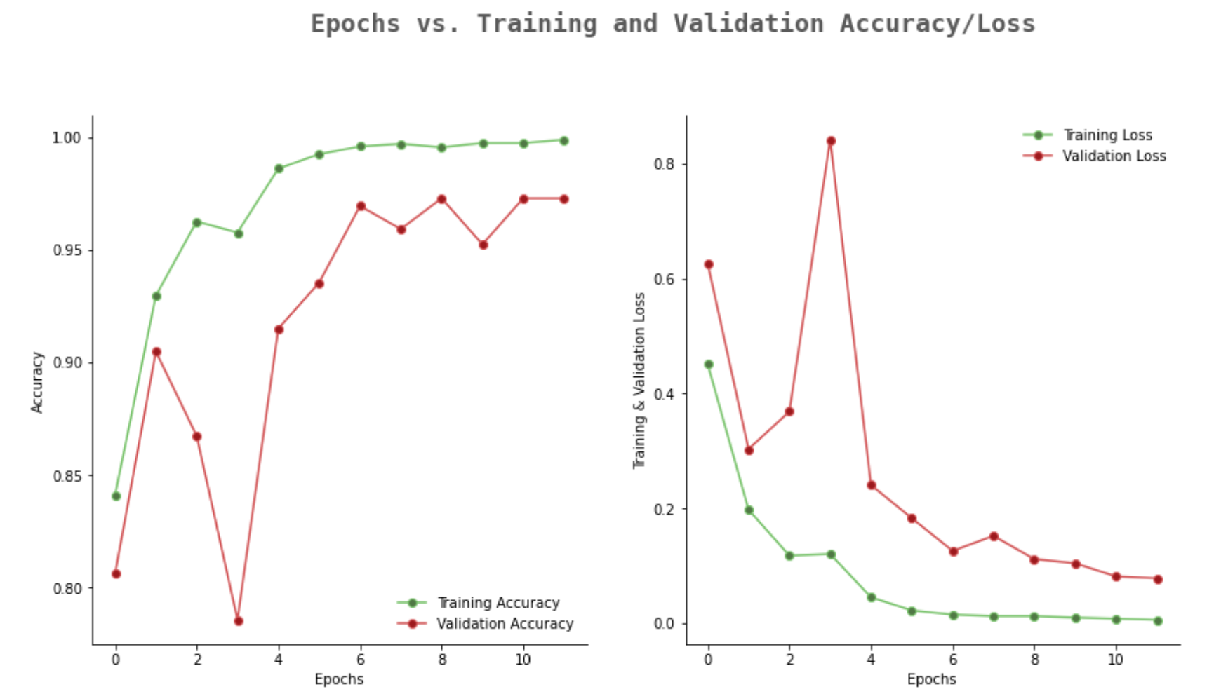
history = model.fit(X_train,y_train,validation_split=0.1, epochs =12, verbose=1, batch_size=32,
callbacks=[tensorboard,checkpoint,reduce_lr])

filterwarnings('ignore')

epochs = [i for i in range(12)]
fig, ax = plt.subplots(1,2,figsize=(14,7))
train_acc = history.history['accuracy']
train_loss = history.history['loss']
val_acc = history.history['val_accuracy']
val_loss = history.history['val_loss']

fig.text(s='Epochs vs. Training and Validation Accuracy/Loss',size=18,fontweight='bold',
fontname='monospace',color=colors_dark[1],y=1,x=0.28,alpha=0.8)

sns.despine()
ax[0].plot(epochs, train_acc, marker='o',markerfacecolor=colors_green[2],color=colors_green[3],
label = 'Training Accuracy')
ax[0].plot(epochs, val_acc, marker='o',markerfacecolor=colors_red[2],color=colors_red[3],
label = 'Validation Accuracy')
ax[0].legend(frameon=False)
ax[0].set_xlabel('Epochs')
ax[0].set_ylabel('Accuracy')

sns.despine()
ax[1].plot(epochs, train_loss, marker='o',markerfacecolor=colors_green[2],color=colors_green[3],
label ='Training Loss')
ax[1].plot(epochs, val_loss, marker='o',markerfacecolor=colors_red[2],color=colors_red[3],
label = 'Validation Loss')
ax[1].legend(frameon=False)
ax[1].set_xlabel('Epochs')
ax[1].set_ylabel('Training & Validation Loss')

fig.show()

预测

使用了argmax函数,因为预测数组中的每一行都包含相应标签的四个值。每行中的最大值描述了4个结果中的预测输出。因此,通过argmax,我能够找出与预测结果相关的索引。

1
2
3
pred = model.predict(X_test)
pred = np.argmax(pred,axis=1)
y_test_new = np.argmax(y_test,axis=1)

评估

  • 0 - Glioma Tumor
  • 1 - No Tumor
  • 2 - Meningioma Tumor
  • 3 - Pituitary Tumor
    1
    print(classification_report(y_test_new,pred))
    结果输出为:
    1
    2
    3
    4
    5
    6
    7
    8
    9
    10
                  precision    recall  f1-score   support

    0 0.98 0.96 0.97 93
    1 0.96 1.00 0.98 51
    2 0.98 0.98 0.98 96
    3 1.00 1.00 1.00 87

    accuracy 0.98 327
    macro avg 0.98 0.98 0.98 327
    weighted avg 0.98 0.98 0.98 327
    1
    2
    3
    4
    5
    6
    7
    fig,ax=plt.subplots(1,1,figsize=(14,7))
    sns.heatmap(confusion_matrix(y_test_new,pred),ax=ax,xticklabels=labels,yticklabels=labels,annot=True,
    cmap=colors_green[::-1],alpha=0.7,linewidths=2,linecolor=colors_dark[3])
    fig.text(s='Heatmap of the Confusion Matrix',size=18,fontweight='bold',
    fontname='monospace',color=colors_dark[1],y=0.92,x=0.28,alpha=0.8)

    plt.show()

我制作了一个组件,可以从本机上传图片并预测MRI扫描是否有脑肿瘤,并对它是哪种肿瘤进行分类。

1
2
3
4
5
6
7
8
9
10
11
12
13
14
15
16
17
18
19
20
21
22
23
24
25
26
27
28
29
30
31
32
33
34
35
36
37
38
def img_pred(upload):
for name, file_info in uploader.value.items():
img = Image.open(io.BytesIO(file_info['content']))
opencvImage = cv2.cvtColor(np.array(img), cv2.COLOR_RGB2BGR)
img = cv2.resize(opencvImage,(150,150))
img = img.reshape(1,150,150,3)
p = model.predict(img)
p = np.argmax(p,axis=1)[0]

if p==0:
p='Glioma Tumor'
elif p==1:
print('The model predicts that there is no tumor')
elif p==2:
p='Meningioma Tumor'
else:
p='Pituitary Tumor'

if p!=1:
print(f'The Model predicts that it is a {p}')

# 您可以在此处单击“上传”按钮来上传图像:
uploader = widgets.FileUpload()
display(uploader)

# 上传图片后,您可以点击下面的预测按钮进行预测:
button = widgets.Button(description='Predict')
out = widgets.Output()
def on_button_clicked(_):
with out:
clear_output()
try:
img_pred(uploader)

except:
print('No Image Uploaded/Invalid Image File')
button.on_click(on_button_clicked)
widgets.VBox([button,out])

CNN的帮助下使用迁移学习进行图像分类,准确率约为98%