介绍 数据集包含25,000张狗和猫的图片。此数据集中的每个图片都有标签作为文件名的一部分。测试文件夹包含12,500张图片,根据数字ID命名。对于测试集中的每个图片,您应该预测该图片是狗/猫的概率(1 = 狗,0 = 猫)。为了解决这个问题,我们将使用预训练模型ResNet-50,仅替换最后一层。
加载包 1 2 3 4 5 6 7 8 9 10 11 12 13 14 15 import os, cv2, randomimport numpy as npimport pandas as pdimport seaborn as snsimport matplotlib.pyplot as pltfrom sklearn.model_selection import train_test_splitfrom sklearn.metrics import classification_reportfrom tqdm import tqdmfrom random import shuffle from IPython.display import SVGfrom keras.utils.vis_utils import model_to_dotfrom keras.utils import plot_modelfrom tensorflow.python.keras.applications import ResNet50from tensorflow.python.keras.models import Sequentialfrom tensorflow.python.keras.layers import Dense, Flatten, GlobalAveragePooling2D
参数 这里我们设置模型中使用的一些参数。图片大小为224。图片存储在两个文件夹中:train和test。有两个图片分类:狗和猫。我们将使用训练数据集的子集(20,000张图片)。训练集中,50%用于训练,50%用于验证。将使用ResNet-50的预训练模型。将使用10个epoch进行训练。
1 2 3 4 5 6 7 8 9 10 11 12 TEST_SIZE = 0.5 RANDOM_STATE = 2018 BATCH_SIZE = 64 NO_EPOCHS = 20 NUM_CLASSES = 2 SAMPLE_SIZE = 20000 PATH = '/kaggle/input/dogs-vs-cats-redux-kernels-edition/' TRAIN_FOLDER = './train/' TEST_FOLDER = './test/' IMG_SIZE = 224 RESNET_WEIGHTS_PATH = '/kaggle/input/resnet50/resnet50_weights_tf_dim_ordering_tf_kernels_notop.h5'
读取数据 我们设置数据集图片列表。设置SAMPLE_SIZE值可以减小/放大训练集的大小。当前SAMPLE_SIZE设置为20,000。
1 2 3 4 5 6 7 8 9 10 11 12 13 import zipfiletrain_image_path = os.path.join(PATH, "train.zip" ) test_image_path = os.path.join(PATH, "test.zip" ) with zipfile.ZipFile(train_image_path,"r" ) as z: z.extractall("." ) with zipfile.ZipFile(test_image_path,"r" ) as z: z.extractall("." ) train_image_list = os.listdir("./train/" )[0 :SAMPLE_SIZE] test_image_list = os.listdir("./test/" )
我们设置一个解析图片名称的函数,从图片名称中提取前3个字母,这给出了图片的标签。它将是一只猫或一只狗。我们使用一个热编码器,为猫存储[1,0],为狗存储[0,1]。
1 2 3 4 def label_pet_image_one_hot_encoder (img ): pet = img.split('.' )[-3 ] if pet == 'cat' : return [1 ,0 ] elif pet == 'dog' : return [0 ,1 ]
我们还定义了一个处理数据(训练集和测试集)的函数。
1 2 3 4 5 6 7 8 9 10 11 12 13 def process_data (data_image_list, DATA_FOLDER, isTrain=True ): data_df = [] for img in tqdm(data_image_list): path = os.path.join(DATA_FOLDER,img) if (isTrain): label = label_pet_image_one_hot_encoder(img) else : label = img.split('.' )[0 ] img = cv2.imread(path,cv2.IMREAD_COLOR) img = cv2.resize(img, (IMG_SIZE,IMG_SIZE)) data_df.append([np.array(img),np.array(label)]) shuffle(data_df) return data_df
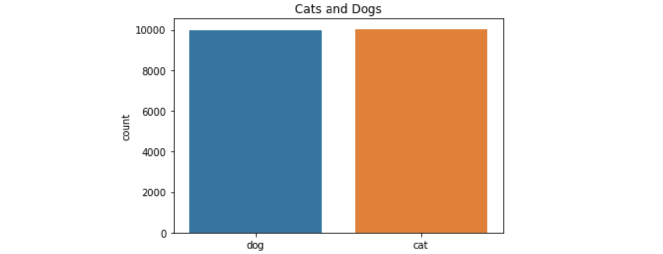
数据分析 类别分布 让我们检查训练数据以检查猫/狗的分布。我们首先展示减少的训练数据中的分割情况。
1 2 3 4 5 6 7 8 def plot_image_list_count (data_image_list ): labels = [] for img in data_image_list: labels.append(img.split('.' )[-3 ]) sns.countplot(labels) plt.title('Cats and Dogs' ) plot_image_list_count(train_image_list)
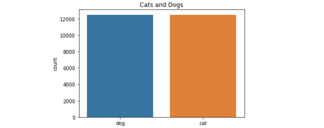
完整的训练集数据的类别分布
1 plot_image_list_count(os.listdir(TRAIN_FOLDER))
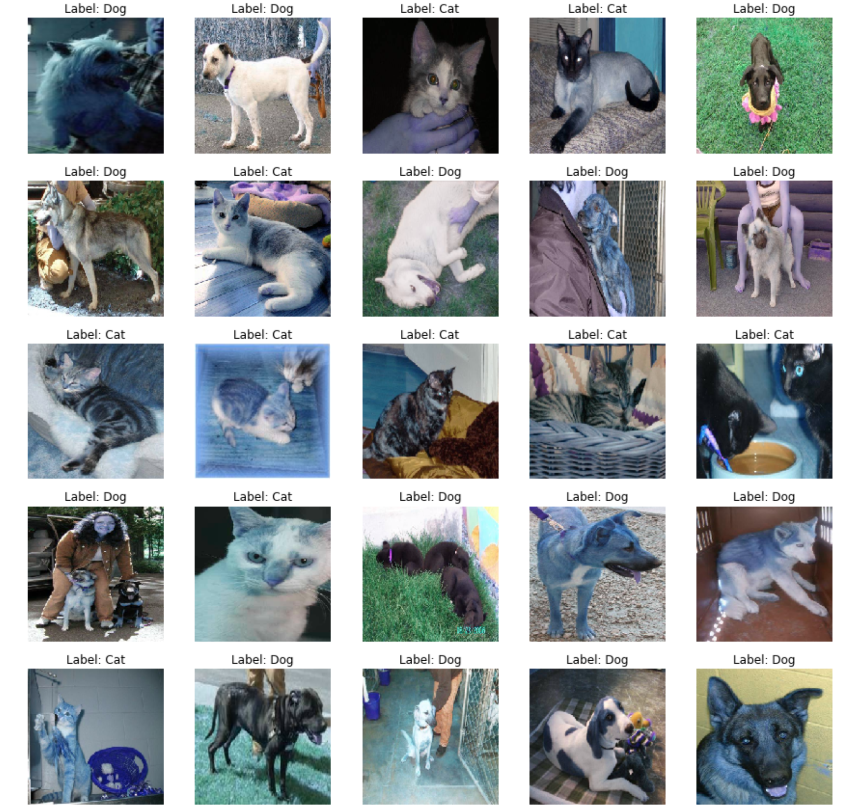
图片样本 让我们重新呈现一些图片。我们从数据集中进行选择。我们将展示训练集中的前25张图片。首先,我们处理训练数据,读取图片并创建包含图片和标签的表格。如果数据是训练集,则标签是通过一次热编码计算得到的标签;如果数据来自测试集,标签将是图片编号。
1 2 3 4 5 6 7 8 9 10 11 12 13 14 15 16 17 18 19 20 train = process_data(train_image_list, TRAIN_FOLDER) def show_images (data, isTest=False ): f, ax = plt.subplots(5 ,5 , figsize=(15 ,15 )) for i,data in enumerate (data[:25 ]): img_num = data[1 ] img_data = data[0 ] label = np.argmax(img_num) if label == 1 : str_label='Dog' elif label == 0 : str_label='Cat' if (isTest): str_label="None" ax[i//5 , i%5 ].imshow(img_data) ax[i//5 , i%5 ].axis('off' ) ax[i//5 , i%5 ].set_title("Label: {}" .format (str_label)) plt.show() show_images(train)
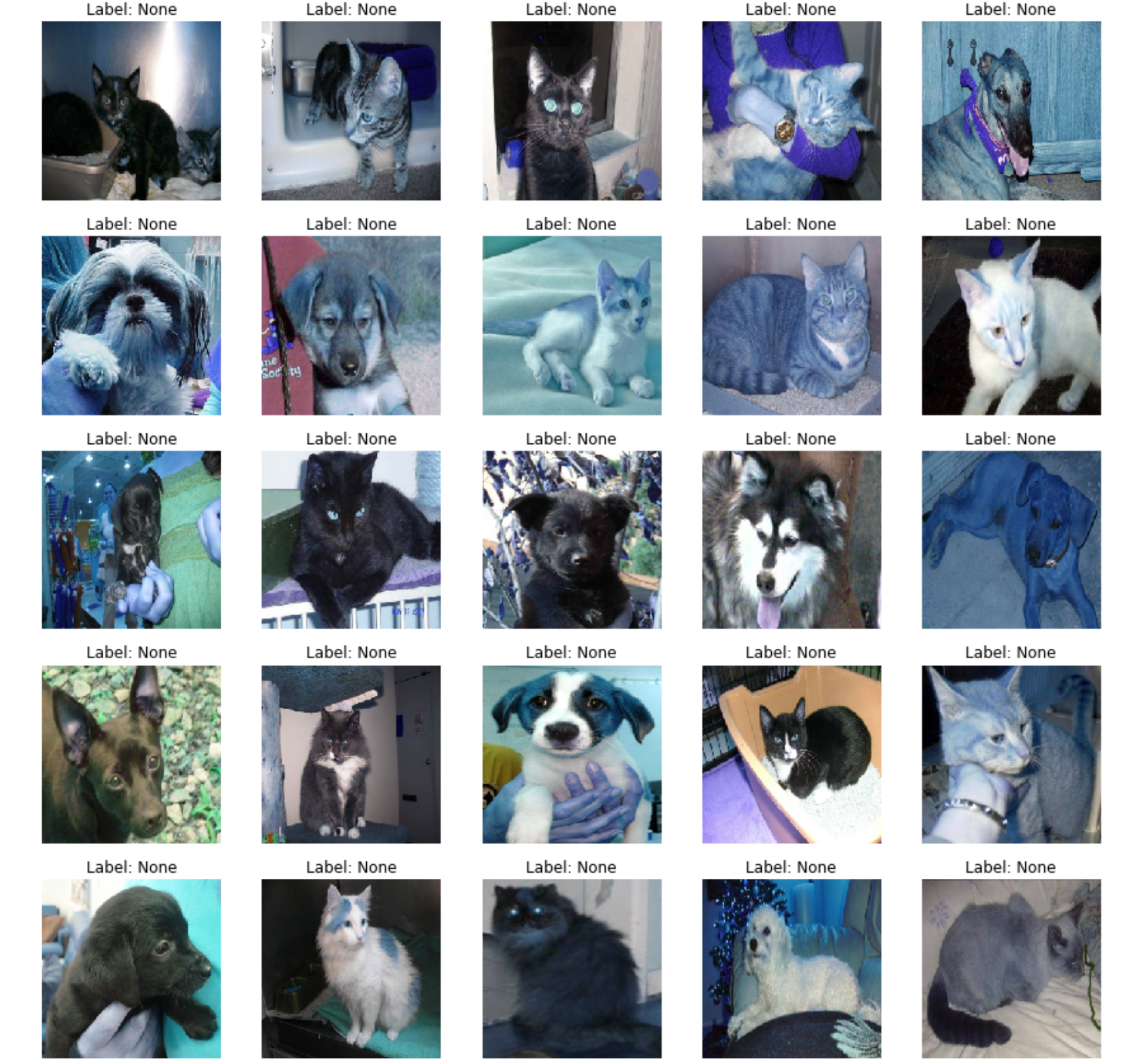
准备测试集
1 2 test = process_data(test_image_list, TEST_FOLDER, False ) show_images(test,True )
Model 准备模型 准备训练数据 1 2 X = np.array([i[0 ] for i in train]).reshape(-1 ,IMG_SIZE,IMG_SIZE,3 ) y = np.array([i[1 ] for i in train])
准备模型 初始化ResNet-50模型,添加一个带有softmax激活函数Dense类型的最后一层。我们还将模型的第一层设置为不可训练,因为ResNet-50模型已经经过训练。
1 2 3 4 5 model = Sequential() model.add(ResNet50(include_top=False , pooling='max' , weights=RESNET_WEIGHTS_PATH)) model.add(Dense(NUM_CLASSES, activation='softmax' )) model.layers[0 ].trainable = True
编译模型 我们使用sigmoid优化、损失函数作为分类交叉熵和度量精度 来编译模型。
1 model.compile (optimizer='sgd' , loss='categorical_crossentropy' , metrics=['accuracy' ])
模型描述 我们绘制模型描述。我们可以看到ResNet-50模型代表模型类型的第一层。
结果输出为:
1 2 3 4 5 6 7 8 9 10 11 _________________________________________________________________ Layer (type ) Output Shape Param ================================================================= resnet50 (Model) (None, 2048) 23587712 _________________________________________________________________ dense (Dense) (None, 2) 4098 ================================================================= Total params: 23,591,810 Trainable params: 23,538,690 Non-trainable params: 53,120 _________________________________________________________________
我们还使用plot_model显示模型图形表示。
1 2 plot_model(model, to_file='model.png' ) SVG(model_to_dot(model).create(prog='dot' , format ='svg' ))
在训练和验证中分割训练数据,我们将数据集分为两部分。一个用于训练集,第二个用于验证集。数据的训练子集将用于训练模型;验证集将用于训练期间的验证。
1 X_train, X_val, y_train, y_val = train_test_split(X, y, test_size=TEST_SIZE, random_state=RANDOM_STATE)
训练模型 1 train_model = model.fit(X_train, y_train,batch_size=BATCH_SIZE,epochs=NO_EPOCHS,verbose=1 ,validation_data=(X_val, y_val))
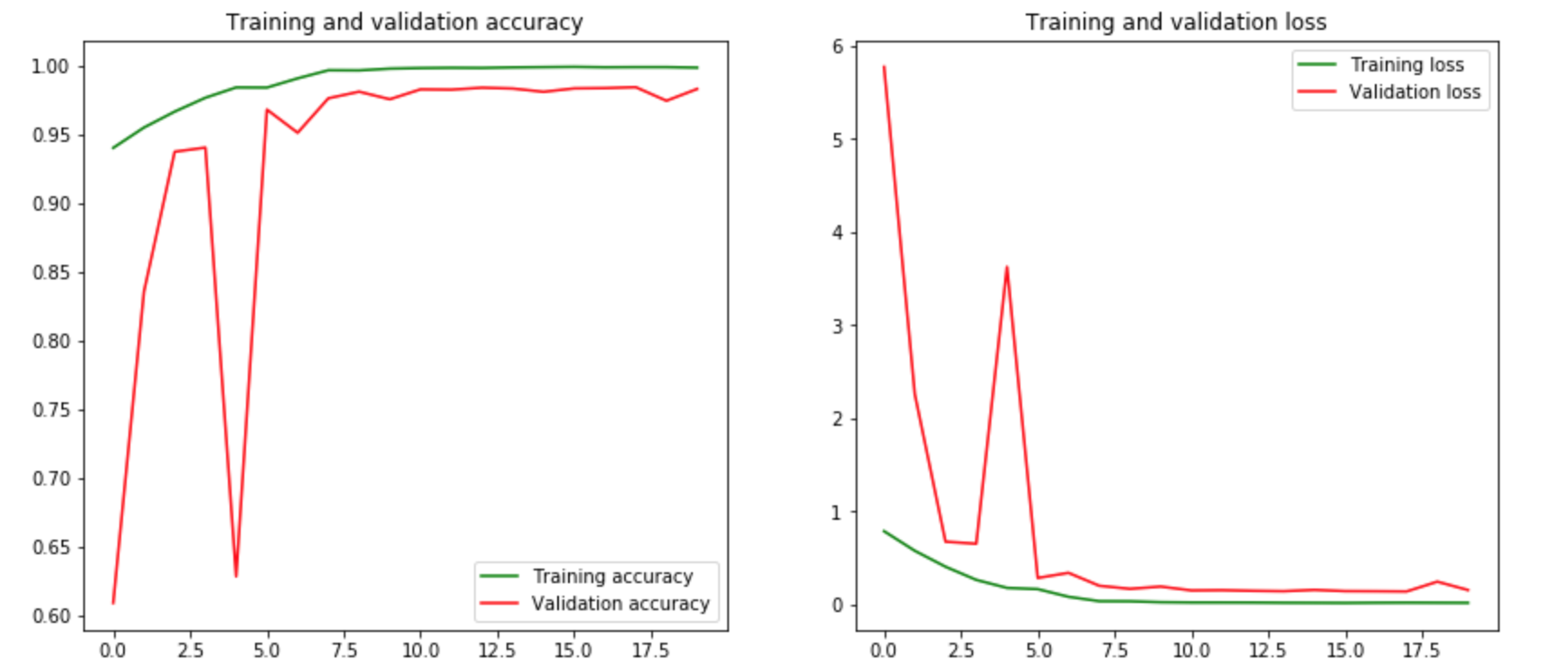
验证准确性和损失 让我们在同一个图上展示训练和验证的准确性。同样,我们将在同一张图上表示训练和验证损失。
1 2 3 4 5 6 7 8 9 10 11 12 13 14 15 16 17 18 19 def plot_accuracy_and_loss (train_model ): hist = train_model.history acc = hist['acc' ] val_acc = hist['val_acc' ] loss = hist['loss' ] val_loss = hist['val_loss' ] epochs = range (len (acc)) f, ax = plt.subplots(1 ,2 , figsize=(14 ,6 )) ax[0 ].plot(epochs, acc, 'g' , label='Training accuracy' ) ax[0 ].plot(epochs, val_acc, 'r' , label='Validation accuracy' ) ax[0 ].set_title('Training and validation accuracy' ) ax[0 ].legend() ax[1 ].plot(epochs, loss, 'g' , label='Training loss' ) ax[1 ].plot(epochs, val_loss, 'r' , label='Validation loss' ) ax[1 ].set_title('Training and validation loss' ) ax[1 ].legend() plt.show() plot_accuracy_and_loss(train_model)
1 2 3 4 5 6 score = model.evaluate(X_val, y_val, verbose=0 ) print ('Validation loss:' , score[0 ])print ('Validation accuracy:' , score[1 ])
每个类别的验证准确性 让我们展示每个类别的验证准确性。我们首先预测验证集的标签。
1 2 3 4 5 6 7 predicted_classes = model.predict_classes(X_val) y_true = np.argmax(y_val,axis=1 ) correct = np.nonzero(predicted_classes==y_true)[0 ] incorrect = np.nonzero(predicted_classes!=y_true)[0 ]
我们为验证集中的图像创建两个索引,正确的和错误的,分别是预测类别正确和错误。我们看到了验证集中正确预测值和错误预测值的数量。显示验证集的分类报告,以及每个类别和总体的准确性。
1 2 3 4 5 6 7 8 9 10 11 target_names = ["Class {}:" .format (i) for i in range (NUM_CLASSES)] print (classification_report(y_true, predicted_classes, target_names=target_names))
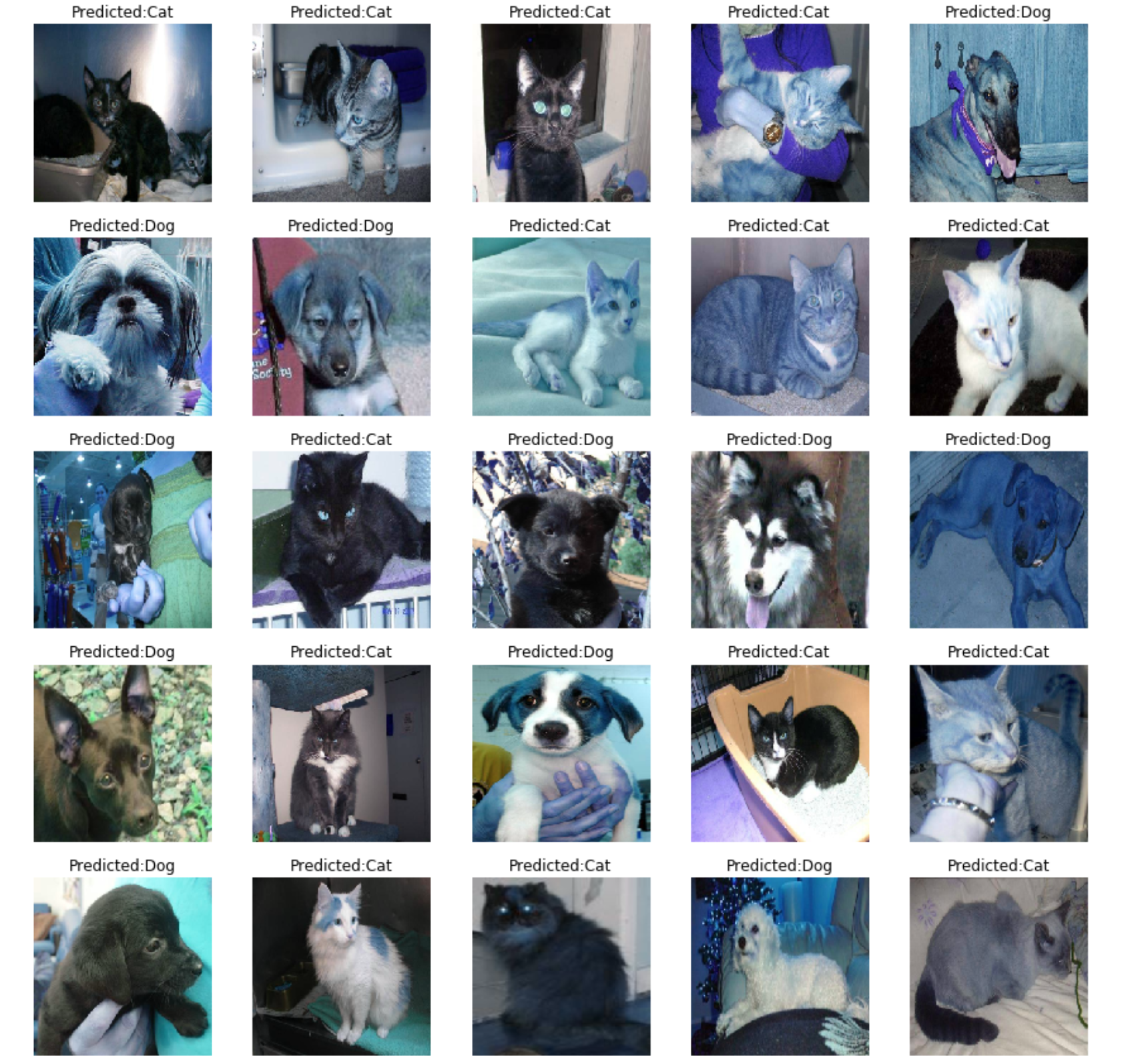
准备提交 显示具有预测类别的测试图片 让我们展示一些具有预测类别的测试图片。为此,我们必须预测这个类别。
1 2 3 4 5 6 7 8 9 10 11 12 13 14 15 16 f, ax = plt.subplots(5 ,5 , figsize=(15 ,15 )) for i,data in enumerate (test[:25 ]): img_num = data[1 ] img_data = data[0 ] orig = img_data data = img_data.reshape(-1 ,IMG_SIZE,IMG_SIZE,3 ) model_out = model.predict([data])[0 ] if np.argmax(model_out) == 1 : str_predicted='Dog' else : str_predicted='Cat' ax[i//5 , i%5 ].imshow(orig) ax[i//5 , i%5 ].axis('off' ) ax[i//5 , i%5 ].set_title("Predicted:{}" .format (str_predicted)) plt.show()
测试数据预测 1 2 3 4 5 6 7 8 9 10 11 12 13 pred_list = [] img_list = [] for img in tqdm(test): img_data = img[0 ] img_idx = img[1 ] data = img_data.reshape(-1 ,IMG_SIZE,IMG_SIZE,3 ) predicted = model.predict([data])[0 ] img_list.append(img_idx) pred_list.append(predicted[1 ]) submission = pd.DataFrame({'id' :img_list , 'label' :pred_list}) submission.to_csv("submission.csv" , index=False )
总结 使用Keras的预训练模型ResNet-50,加上顶部添加了softmax激活的密集模型,并使用减少的集合进行训练,我们能够在验证准确性方面获得相当好的模型。该模型用于预测独立测试集中的图片分类类别,使用新数据测试预测的准确性并提交预测结果。