介绍 我们将使用TensorFlow和Keras来构建计算机视觉模型,并使用TPU来训练我们的模型并进行预测。
张量处理单元 (TPU) Tensor处理单元(TPU)是专门用于深度学习任务的硬件加速器。
设置环境 1 2 3 4 5 6 7 8 9 10 import math, re, osimport tensorflow as tfimport numpy as npimport pandas as pdimport matplotlib.pyplot as pltfrom kaggle_datasets import KaggleDatasetsfrom tensorflow import kerasfrom functools import partialfrom sklearn.model_selection import train_test_splitprint ("Tensorflow version " + tf.__version__)
检测TPU 我们在这里使用代码确保我们将通过TPU发送数据。您正在寻找的是“副本数量:8”的打印输出,对应于TPU的8个核心。如果您的打印输出显示“副本数:1”,则您的笔记本电脑中可能没有启用TPU。要启用TPU,请导航至右侧面板并单击加速器。从下拉列表中选择TPU。
1 2 3 4 5 6 7 8 9 try : tpu = tf.distribute.cluster_resolver.TPUClusterResolver() print ('Device:' , tpu.master()) tf.config.experimental_connect_to_cluster(tpu) tf.tpu.experimental.initialize_tpu_system(tpu) strategy = tf.distribute.experimental.TPUStrategy(tpu) except : strategy = tf.distribute.get_strategy() print ('Number of replicas:' , strategy.num_replicas_in_sync)
结果输出为:
1 2 Device: grpc://10.0.0.2:8470 Number of replicas: 8
设置变量 如果您碰巧使用的是私有数据集,您还需要确保您的笔记本上附加了Google Cloud软件开发套件(SDK)。您可以在笔记本顶部的附加组件下拉菜单下找到Google Cloud SDK。您可以在此处找到Google Cloud软件开发套件(SDK)的文档。
1 2 3 4 5 6 AUTOTUNE = tf.data.experimental.AUTOTUNE GCS_PATH = KaggleDatasets().get_gcs_path() BATCH_SIZE = 16 * strategy.num_replicas_in_sync IMAGE_SIZE = [512 , 512 ] CLASSES = ['0' , '1' , '2' , '3' , '4' ] EPOCHS = 25
加载数据 我们正在处理的数据已被格式化为TFRecords,这是一种用于存储二进制记录序列的格式。TFRecords与TPU配合得非常好,允许我们通过TPU发送少量大文件进行处理。由于我们的数据仅包含训练和测试图像,因此我们将使用train_test_split()函数将训练数据分为训练数据和验证数据。
解码数据 在下面的代码块中,我们将设置一系列函数,使我们能够将图像转换为张量,以便我们可以在模型中使用它们。我们还将标准化我们的数据。我们的图像使用范围为[0, 255] 的“红、蓝、绿(RBG)”比例,通过对其进行标准化,我们将每个像素的值设置为[0, 1]范围内的数字 。
1 2 3 4 5 def decode_image (image ): image = tf.image.decode_jpeg(image, channels=3 ) image = tf.cast(image, tf.float32) / 255.0 image = tf.reshape(image, [*IMAGE_SIZE, 3 ]) return image
如果您回想一下机器学习,您可能还记得我们如何设置X和y等变量,代表我们的特征X和预测目标y。这段代码完成了类似的事情,尽管我们的特征不是使用标签X和y,而是由术语图像表示,而我们的预测目标由术语目标表示。您可能还注意到此函数考虑了未标记的图像。这是因为我们的测试图像没有任何标签。
1 2 3 4 5 6 7 8 9 10 11 12 13 14 15 def read_tfrecord (example, labeled ): tfrecord_format = { "image" : tf.io.FixedLenFeature([], tf.string), "target" : tf.io.FixedLenFeature([], tf.int64) } if labeled else { "image" : tf.io.FixedLenFeature([], tf.string), "image_name" : tf.io.FixedLenFeature([], tf.string) } example = tf.io.parse_single_example(example, tfrecord_format) image = decode_image(example['image' ]) if labeled: label = tf.cast(example['target' ], tf.int32) return image, label idnum = example['image_name' ] return image, idnum
我们将使用以下函数来加载数据集。TPU的优点之一是我们可以同时在TPU上运行多个文件,这就是使用TPU的速度优势。为了利用这一点,我们希望确保我们在数据流入时立即使用它,而不是创建数据流瓶颈。
1 2 3 4 5 6 7 8 def load_dataset (filenames, labeled=True , ordered=False ): ignore_order = tf.data.Options() if not ordered: ignore_order.experimental_deterministic = False dataset = tf.data.TFRecordDataset(filenames, num_parallel_reads=AUTOTUNE) dataset = dataset.with_options(ignore_order) dataset = dataset.map (partial(read_tfrecord, labeled=labeled), num_parallel_calls=AUTOTUNE) return dataset
使用train_test_split()的注意事项 虽然我使用train_test_split()创建训练和验证数据集,但请考虑探索交叉验证 。
1 2 3 4 5 6 TRAINING_FILENAMES, VALID_FILENAMES = train_test_split( tf.io.gfile.glob(GCS_PATH + '/train_tfrecords/ld_train*.tfrec' ), test_size=0.35 , random_state=5 ) TEST_FILENAMES = tf.io.gfile.glob(GCS_PATH + '/test_tfrecords/ld_test*.tfrec' )
添加增强 在这里我通过TensorFlow应用了可用的增强功能。您可以在TensorFlow tf.image文档中阅读有关这些增强功能的更多信息。
1 2 3 4 5 def data_augment (image, label ): image = tf.image.random_flip_left_right(image) return image, label
定义数据加载方法 以下函数将用于加载我们的训练、验证和测试 数据集,以及打印每个数据集中的图像数量。
1 2 3 4 5 6 7 8 9 10 11 12 13 14 15 16 17 18 19 20 21 22 23 24 25 26 27 28 29 30 31 32 33 def get_training_dataset (): dataset = load_dataset(TRAINING_FILENAMES, labeled=True ) dataset = dataset.map (data_augment, num_parallel_calls=AUTOTUNE) dataset = dataset.repeat() dataset = dataset.shuffle(2048 ) dataset = dataset.batch(BATCH_SIZE) dataset = dataset.prefetch(AUTOTUNE) return dataset def get_validation_dataset (ordered=False ): dataset = load_dataset(VALID_FILENAMES, labeled=True , ordered=ordered) dataset = dataset.batch(BATCH_SIZE) dataset = dataset.cache() dataset = dataset.prefetch(AUTOTUNE) return dataset def get_test_dataset (ordered=False ): dataset = load_dataset(TEST_FILENAMES, labeled=False , ordered=ordered) dataset = dataset.batch(BATCH_SIZE) dataset = dataset.prefetch(AUTOTUNE) return dataset def count_data_items (filenames ): n = [int (re.compile (r"-([0-9]*)\." ).search(filename).group(1 )) for filename in filenames] return np.sum (n) NUM_TRAINING_IMAGES = count_data_items(TRAINING_FILENAMES) NUM_VALIDATION_IMAGES = count_data_items(VALID_FILENAMES) NUM_TEST_IMAGES = count_data_items(TEST_FILENAMES) print ('Dataset: {} training images, {} validation images, {} (unlabeled) test images' .format ( NUM_TRAINING_IMAGES, NUM_VALIDATION_IMAGES, NUM_TEST_IMAGES))
结果输出为:
1 Dataset: 13380 training images, 8017 validation images, 1 (unlabeled) test images
简短的探索性数据分析(EDA) 首先,我们将打印三个数据集样本的形状和标签:
1 2 3 4 5 6 7 8 9 10 11 12 print ("Training data shapes:" )for image, label in get_training_dataset().take(3 ): print (image.numpy().shape, label.numpy().shape) print ("Training data label examples:" , label.numpy())print ("Validation data shapes:" )for image, label in get_validation_dataset().take(3 ): print (image.numpy().shape, label.numpy().shape) print ("Validation data label examples:" , label.numpy())print ("Test data shapes:" )for image, idnum in get_test_dataset().take(3 ): print (image.numpy().shape, idnum.numpy().shape) print ("Test data IDs:" , idnum.numpy().astype('U' ))
结果输出为:
1 2 3 4 5 6 7 8 9 10 11 12 13 14 15 16 17 18 19 Training data shapes: (128, 512, 512, 3) (128,) (128, 512, 512, 3) (128,) (128, 512, 512, 3) (128,) Training data label examples: [3 4 4 3 3 2 4 3 3 3 1 3 3 3 3 3 3 3 4 3 2 1 4 1 1 2 3 3 1 2 3 4 4 3 1 1 3 4 3 3 4 4 3 3 3 3 3 3 0 3 2 3 4 2 3 3 3 1 3 3 3 3 3 3 4 2 3 3 3 3 3 3 3 3 3 3 1 3 3 3 3 3 1 3 3 1 3 1 3 2 3 3 3 3 4 0 3 3 4 4 4 3 3 3 3 3 3 0 3 4 3 3 3 0 1 3 3 3 3 2 3 3 3 3 3 3 3 3] Validation data shapes: (128, 512, 512, 3) (128,) (128, 512, 512, 3) (128,) (128, 512, 512, 3) (128,) Validation data label examples: [3 3 3 1 3 3 3 3 4 0 4 3 0 2 4 3 3 3 3 1 3 3 2 3 3 3 1 2 3 3 1 3 0 3 3 1 3 4 3 3 3 3 4 4 2 3 2 2 3 3 2 3 3 1 1 3 4 3 4 3 4 3 3 3 3 3 2 1 0 4 3 3 3 3 3 0 0 2 3 3 3 2 3 3 1 3 3 3 3 3 4 3 0 3 3 2 1 3 3 3 4 4 4 3 4 3 3 3 2 4 1 3 4 3 4 3 2 0 1 3 3 2 2 3 3 2 3 0] Test data shapes: (1, 512, 512, 3) (1,) Test data IDs: ['2216849948.jpg' ]
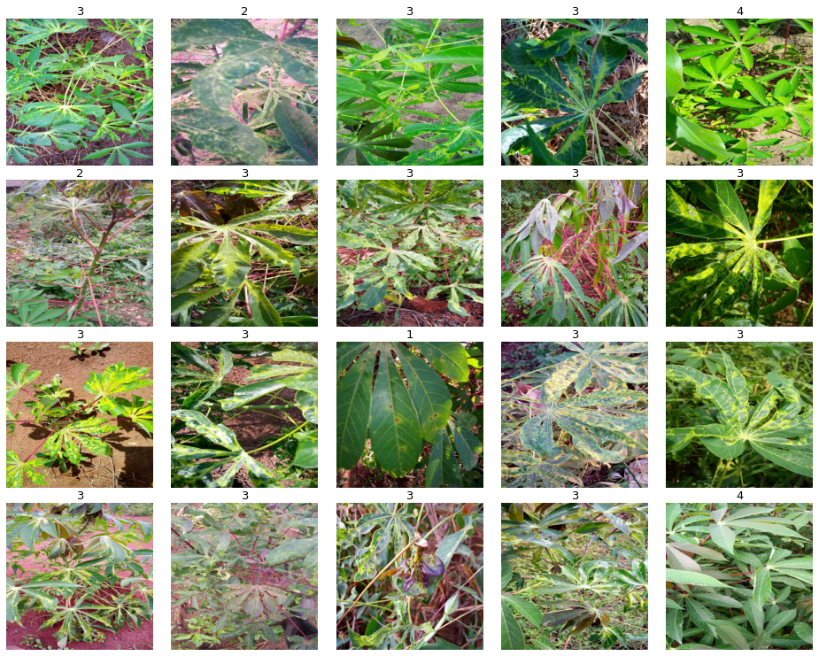
以下代码块设置了一系列将打印出图像网格的函数。图像网格将包含图像及其相应的标签。
1 2 3 4 5 6 7 8 9 10 11 12 13 14 15 16 17 18 19 20 21 22 23 24 25 26 27 28 29 30 31 32 33 34 35 36 37 38 39 40 41 42 43 44 45 46 47 48 49 50 51 52 53 54 55 56 57 58 59 60 61 62 63 64 65 66 67 68 69 70 71 72 73 74 75 76 np.set_printoptions(threshold=15 , linewidth=80 ) def batch_to_numpy_images_and_labels (data ): images, labels = data numpy_images = images.numpy() numpy_labels = labels.numpy() if numpy_labels.dtype == object : numpy_labels = [None for _ in enumerate (numpy_images)] return numpy_images, numpy_labels def title_from_label_and_target (label, correct_label ): if correct_label is None : return CLASSES[label], True correct = (label == correct_label) return "{} [{}{}{}]" .format (CLASSES[label], 'OK' if correct else 'NO' , u"\u2192" if not correct else '' , CLASSES[correct_label] if not correct else '' ), correct def display_one_plant (image, title, subplot, red=False , titlesize=16 ): plt.subplot(*subplot) plt.axis('off' ) plt.imshow(image) if len (title) > 0 : plt.title(title, fontsize=int (titlesize) if not red else int (titlesize/1.2 ), color='red' if red else 'black' , fontdict={'verticalalignment' :'center' }, pad=int (titlesize/1.5 )) return (subplot[0 ], subplot[1 ], subplot[2 ]+1 ) def display_batch_of_images (databatch, predictions=None ): """This will work with: display_batch_of_images(images) display_batch_of_images(images, predictions) display_batch_of_images((images, labels)) display_batch_of_images((images, labels), predictions) """ images, labels = batch_to_numpy_images_and_labels(databatch) if labels is None : labels = [None for _ in enumerate (images)] rows = int (math.sqrt(len (images))) cols = len (images)//rows FIGSIZE = 13.0 SPACING = 0.1 subplot=(rows,cols,1 ) if rows < cols: plt.figure(figsize=(FIGSIZE,FIGSIZE/cols*rows)) else : plt.figure(figsize=(FIGSIZE/rows*cols,FIGSIZE)) for i, (image, label) in enumerate (zip (images[:rows*cols], labels[:rows*cols])): title = '' if label is None else CLASSES[label] correct = True if predictions is not None : title, correct = title_from_label_and_target(predictions[i], label) dynamic_titlesize = FIGSIZE*SPACING/max (rows,cols)*40 +3 subplot = display_one_plant(image, title, subplot, not correct, titlesize=dynamic_titlesize) plt.tight_layout() if label is None and predictions is None : plt.subplots_adjust(wspace=0 , hspace=0 ) else : plt.subplots_adjust(wspace=SPACING, hspace=SPACING) plt.show() training_dataset = get_training_dataset() training_dataset = training_dataset.unbatch().batch(20 ) train_batch = iter (training_dataset) display_batch_of_images(next (train_batch))
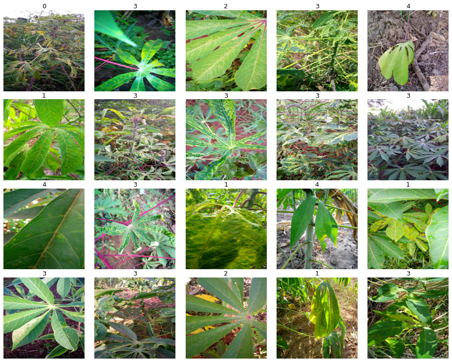
您还可以修改上面的代码来查看验证和测试数据,如下所示:
1 2 3 4 5 6 7 validation_dataset = get_validation_dataset() validation_dataset = validation_dataset.unbatch().batch(20 ) valid_batch = iter (validation_dataset) display_batch_of_images(next (valid_batch))
1 2 3 4 5 6 7 testing_dataset = get_test_dataset() testing_dataset = testing_dataset.unbatch().batch(20 ) test_batch = iter (testing_dataset) display_batch_of_images(next (test_batch))
构建模型 学习率计划 在这里我创建了一个学习率计划 ,主要使用Keras指数衰减学习率计划 程序文档中的默认值(我确实更改了initial_learning_rate。您可以调整下面的学习率 计划程序,并在 Keras学习率计划API中详细了解可用的其他类型的计划程序。
1 2 3 4 lr_scheduler = keras.optimizers.schedules.ExponentialDecay( initial_learning_rate=1e-5 , decay_steps=10000 , decay_rate=0.9 )
构建我们的模型 为了确保我们的模型在TPU上进行训练,我们使用Strategy.scope()来构建它。该模型是使用迁移学习构建的,这意味着我们有一个预先训练的模型(ResNet50)作为我们的基础模型,然后使用tf.keras.Sequential构建可定制的模型。如果您是迁移学习新手,我建议将base_model.trainable设置为False,但鼓励您更改正在使用的基本模型(tf.keras.applications模块文档中提供了更多选项)以及迭代定制模型。
请注意 ,我们使用稀疏_分类_交叉熵作为损失函数,因为我们没有对标签进行一次性编码。
1 2 3 4 5 6 7 8 9 10 11 12 13 14 15 16 17 18 19 20 with strategy.scope(): img_adjust_layer = tf.keras.layers.Lambda(tf.keras.applications.resnet50.preprocess_input, input_shape=[*IMAGE_SIZE, 3 ]) base_model = tf.keras.applications.ResNet50(weights='imagenet' , include_top=False ) base_model.trainable = False model = tf.keras.Sequential([ tf.keras.layers.BatchNormalization(renorm=True ), img_adjust_layer, base_model, tf.keras.layers.GlobalAveragePooling2D(), tf.keras.layers.Dense(8 , activation='relu' ), tf.keras.layers.Dense(len (CLASSES), activation='softmax' ) ]) model.compile ( optimizer=tf.keras.optimizers.Adam(learning_rate=lr_scheduler, epsilon=0.001 ), loss='sparse_categorical_crossentropy' , metrics=['sparse_categorical_accuracy' ])
训练模型 当我们的模型正在训练时,您将看到每个时期的打印输出,并且还可以通过单击笔记本右上角工具栏中的TPU指标来监控TPU使用情况。
1 2 3 4 5 6 7 8 9 10 11 12 train_dataset = get_training_dataset() valid_dataset = get_validation_dataset() STEPS_PER_EPOCH = NUM_TRAINING_IMAGES // BATCH_SIZE VALID_STEPS = NUM_VALIDATION_IMAGES // BATCH_SIZE history = model.fit(train_dataset, steps_per_epoch=STEPS_PER_EPOCH, epochs=EPOCHS, validation_data=valid_dataset, validation_steps=VALID_STEPS)
结果输出为:
1 2 3 4 5 6 7 8 9 10 11 12 13 14 15 16 17 18 19 20 21 22 23 24 25 26 27 28 29 30 31 32 33 34 35 36 37 38 39 40 41 42 43 44 45 46 47 48 49 50 Epoch 1/25 104/104 [==============================] - 53s 506ms/step - loss: 2.0801 - sparse_categorical_accuracy: 0.1090 - val_loss: 2.0553 - val_sparse_categorical_accuracy: 0.1159 Epoch 2/25 104/104 [==============================] - 37s 358ms/step - loss: 2.0020 - sparse_categorical_accuracy: 0.1087 - val_loss: 1.8630 - val_sparse_categorical_accuracy: 0.1173 Epoch 3/25 104/104 [==============================] - 37s 359ms/step - loss: 1.6200 - sparse_categorical_accuracy: 0.1618 - val_loss: 1.4386 - val_sparse_categorical_accuracy: 0.3606 Epoch 4/25 104/104 [==============================] - 36s 349ms/step - loss: 1.3472 - sparse_categorical_accuracy: 0.5534 - val_loss: 1.3035 - val_sparse_categorical_accuracy: 0.6077 Epoch 5/25 104/104 [==============================] - 36s 349ms/step - loss: 1.2585 - sparse_categorical_accuracy: 0.6200 - val_loss: 1.2406 - val_sparse_categorical_accuracy: 0.6139 Epoch 6/25 104/104 [==============================] - 36s 348ms/step - loss: 1.2070 - sparse_categorical_accuracy: 0.6240 - val_loss: 1.2035 - val_sparse_categorical_accuracy: 0.6145 Epoch 7/25 104/104 [==============================] - 36s 350ms/step - loss: 1.1712 - sparse_categorical_accuracy: 0.6267 - val_loss: 1.1804 - val_sparse_categorical_accuracy: 0.6154 Epoch 8/25 104/104 [==============================] - 36s 348ms/step - loss: 1.1624 - sparse_categorical_accuracy: 0.6224 - val_loss: 1.1666 - val_sparse_categorical_accuracy: 0.6155 Epoch 9/25 104/104 [==============================] - 37s 356ms/step - loss: 1.1468 - sparse_categorical_accuracy: 0.6227 - val_loss: 1.1563 - val_sparse_categorical_accuracy: 0.6159 Epoch 10/25 104/104 [==============================] - 37s 351ms/step - loss: 1.1336 - sparse_categorical_accuracy: 0.6248 - val_loss: 1.1466 - val_sparse_categorical_accuracy: 0.6162 Epoch 11/25 104/104 [==============================] - 36s 349ms/step - loss: 1.1301 - sparse_categorical_accuracy: 0.6218 - val_loss: 1.1385 - val_sparse_categorical_accuracy: 0.6163 Epoch 12/25 104/104 [==============================] - 36s 349ms/step - loss: 1.1215 - sparse_categorical_accuracy: 0.6242 - val_loss: 1.1308 - val_sparse_categorical_accuracy: 0.6172 Epoch 13/25 104/104 [==============================] - 36s 346ms/step - loss: 1.1141 - sparse_categorical_accuracy: 0.6228 - val_loss: 1.1230 - val_sparse_categorical_accuracy: 0.6186 Epoch 14/25 104/104 [==============================] - 36s 348ms/step - loss: 1.1048 - sparse_categorical_accuracy: 0.6274 - val_loss: 1.1158 - val_sparse_categorical_accuracy: 0.6202 Epoch 15/25 104/104 [==============================] - 36s 347ms/step - loss: 1.0972 - sparse_categorical_accuracy: 0.6266 - val_loss: 1.1087 - val_sparse_categorical_accuracy: 0.6216 Epoch 16/25 104/104 [==============================] - 36s 349ms/step - loss: 1.0927 - sparse_categorical_accuracy: 0.6268 - val_loss: 1.1022 - val_sparse_categorical_accuracy: 0.6232 Epoch 17/25 104/104 [==============================] - 36s 346ms/step - loss: 1.0822 - sparse_categorical_accuracy: 0.6290 - val_loss: 1.0959 - val_sparse_categorical_accuracy: 0.6239 Epoch 18/25 104/104 [==============================] - 36s 350ms/step - loss: 1.0824 - sparse_categorical_accuracy: 0.6261 - val_loss: 1.0904 - val_sparse_categorical_accuracy: 0.6259 Epoch 19/25 104/104 [==============================] - 36s 349ms/step - loss: 1.0784 - sparse_categorical_accuracy: 0.6274 - val_loss: 1.0846 - val_sparse_categorical_accuracy: 0.6279 Epoch 20/25 104/104 [==============================] - 36s 348ms/step - loss: 1.0600 - sparse_categorical_accuracy: 0.6345 - val_loss: 1.0793 - val_sparse_categorical_accuracy: 0.6282 Epoch 21/25 104/104 [==============================] - 36s 349ms/step - loss: 1.0663 - sparse_categorical_accuracy: 0.6288 - val_loss: 1.0737 - val_sparse_categorical_accuracy: 0.6280 Epoch 22/25 104/104 [==============================] - 36s 348ms/step - loss: 1.0601 - sparse_categorical_accuracy: 0.6294 - val_loss: 1.0692 - val_sparse_categorical_accuracy: 0.6287 Epoch 23/25 104/104 [==============================] - 36s 348ms/step - loss: 1.0517 - sparse_categorical_accuracy: 0.6325 - val_loss: 1.0649 - val_sparse_categorical_accuracy: 0.6288 Epoch 24/25 104/104 [==============================] - 36s 347ms/step - loss: 1.0456 - sparse_categorical_accuracy: 0.6336 - val_loss: 1.0601 - val_sparse_categorical_accuracy: 0.6289 Epoch 25/25 104/104 [==============================] - 36s 347ms/step - loss: 1.0445 - sparse_categorical_accuracy: 0.6330 - val_loss: 1.0554 - val_sparse_categorical_accuracy: 0.6298
通过model.summary(),我们将看到每个层的打印输出、它们相应的形状以及相关的参数数量。请注意,在打印输出的底部,我们将看到有关总参数、可训练参数和不可训练参数的信息。因为我们使用的是预训练模型,所以我们预计会有大量不可训练的参数(因为权重已经在预训练模型中分配)。
结果输出为:
1 2 3 4 5 6 7 8 9 10 11 12 13 14 15 16 17 18 19 20 Model: "sequential" _________________________________________________________________ Layer (type ) Output Shape Param ================================================================= batch_normalization (BatchNo multiple 21 _________________________________________________________________ lambda (Lambda) multiple 0 _________________________________________________________________ resnet50 (Model) (None, None, None, 2048) 23587712 _________________________________________________________________ global_average_pooling2d (Gl multiple 0 _________________________________________________________________ dense (Dense) multiple 16392 _________________________________________________________________ dense_1 (Dense) multiple 45 ================================================================= Total params: 23,604,170 Trainable params: 16,443 Non-trainable params: 23,587,727 _________________________________________________________________
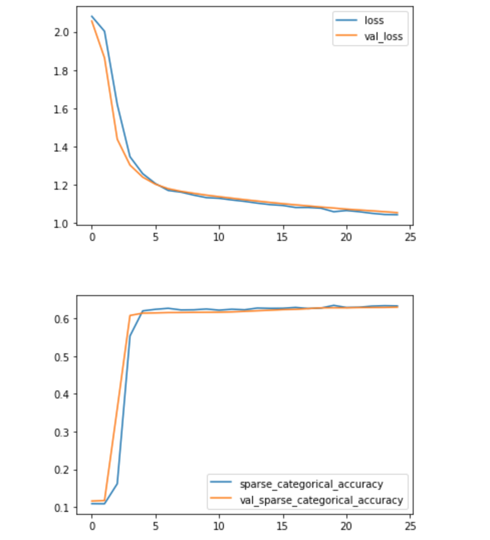
评估我们的模型 提供第一块代码是为了向您展示第二块代码中的变量来自何处。正如您所看到的,该模型还有很大的改进空间,但由于我们使用TPU并且训练时间相对较短,因此我们能够相当快速地迭代我们的模型。
1 2 print (history.history.keys())
结果输出为:
1 dict_keys(['loss' , 'sparse_categorical_accuracy' , 'val_loss' , 'val_sparse_categorical_accuracy' ])
1 2 3 4 history_frame = pd.DataFrame(history.history) history_frame.loc[:, ['loss' , 'val_loss' ]].plot() history_frame.loc[:, ['sparse_categorical_accuracy' , 'val_sparse_categorical_accuracy' ]].plot();
做出预测 现在我们已经训练了我们的模型,我们可以用它来进行预测!
1 2 3 4 5 6 7 8 9 10 11 12 13 def to_float32 (image, label ): return tf.cast(image, tf.float32), label test_ds = get_test_dataset(ordered=True ) test_ds = test_ds.map (to_float32) print ('Computing predictions...' )test_images_ds = testing_dataset test_images_ds = test_ds.map (lambda image, idnum: image) probabilities = model.predict(test_images_ds) predictions = np.argmax(probabilities, axis=-1 ) print (predictions)
创建提交文件 现在我们已经训练了模型并做出了预测。您可以运行下面的代码来获取您的提交文件。
1 2 3 4 5 print ('Generating submission.csv file...' )test_ids_ds = test_ds.map (lambda image, idnum: idnum).unbatch() test_ids = next (iter (test_ids_ds.batch(NUM_TEST_IMAGES))).numpy().astype('U' ) np.savetxt('submission.csv' , np.rec.fromarrays([test_ids, predictions]), fmt=['%s' , '%d' ], delimiter=',' , header='id,label' , comments='' ) !head submission.csv
结果输出为:
1 2 3 4 Generating submission.csv file... id ,label2216849948.jpg,3 ......