基于机器学习 — 花瓣图像分类(TensorFlow & Keras)
介绍
构建一个机器学习模型,根据图像对104种花朵进行分类。您将学习如何在Keras中构建图像分类器并在张量处理单元(TPU)上对其进行训练。
第1步:导入包
我们首先导入几个Python包。
1 | import math, re, os |
第2步:分布式策略
TPU有八个不同的核心,每个核心都充当自己的加速器。(TPU有点像一台机器上有八个GPU)我们告诉TensorFlow如何通过分布式策略同时使用所有这些核心。
1 | # Detect TPU, return appropriate distribution strategy |
创建神经网络模型时,我们将使用分布式策略。然后,TensorFlow将通过创建八个不同的模型副本(每个核心一个)在八个TPU核心之间分配训练。
第3步:加载数据
获取GCS路径
与TPU一起使用时,数据集需要存储在Google Cloud Storage存储桶中。您可以通过提供路径来使用任何公共GCS存储桶中的数据,就像使用“/kaggle/input”中的数据一样。下面将检索数据集的GCS路径。
1 | from kaggle_datasets import KaggleDatasets |
加载数据
与TPU一起使用时,数据集通常会序列化为TFRecord。这是一种方便将数据分发到每个TPU核心的格式。我们隐藏了读取数据集TFRecords的单元格,因为该过程有点长。您可以稍后再回来查看有关自己的数据集与TPU结合使用的一些指导。
1 | IMAGE_SIZE = [512, 512] |
创建数据管道
在最后一步中,我们将使用tf.data API为每个训练、验证和测试拆分定义高效的数据管道。
1 | def data_augment(image, label): |
下一个单元将创建我们将在训练和推理期间与Keras一起使用的数据集。请注意我们如何将批次的大小调整为TPU核心的数量。
1 | # Define the batch size. This will be 16 with TPU off and 128 (=16*8) with TPU on |
结果输出为:
1 | Training: <PrefetchDataset shapes: ((None, 512, 512, 3), (None,)), types: (tf.float32, tf.int32)> |
这些数据集是tf.data.Dataset对象。您可以将TensorFlow中的数据集视为数据记录流。训练集和验证集是(image, label)对的流。
1 | np.set_printoptions(threshold=15, linewidth=80) |
结果输出为:
1 | Training data shapes: |
测试集是(image,idnum)对的流;这里的idnum是为图像提供的唯一标识符,稍后我们以csv文件形式提交时将使用该标识符。
1 | print("Test data shapes:") |
结果输出为:
1 | Test data shapes: |
第 4 步:探索数据
让我们花点时间看一下数据集中的一些图像。
1 | from matplotlib import pyplot as plt |
您可以使用我们的另一个辅助函数显示数据集中的一批图像。下一个单元格会将数据集转换为20个图像批次的迭代器。
1 | ds_iter = iter(ds_train.unbatch().batch(20)) |
使用Python next函数输出流中的下一批,并使用辅助函数显示它。
1 | one_batch = next(ds_iter) |
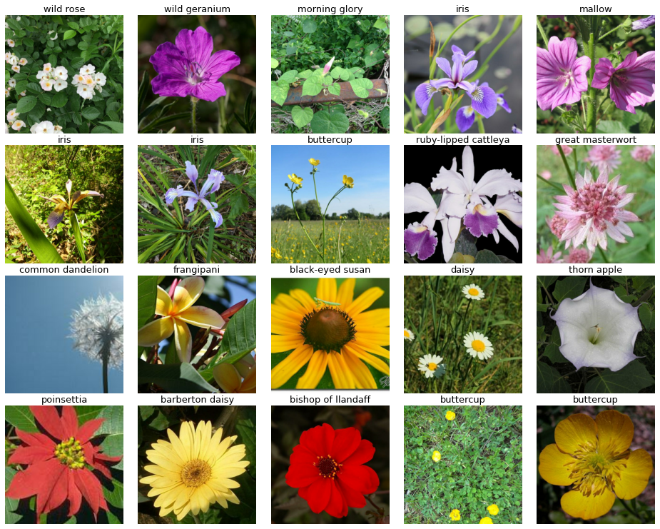
通过在单独的单元格中定义ds_iter和one_batch,您只需重新运行上面的单元格即可看到一批新图像。
第5步:定义模型
现在我们准备创建一个用于图像分类的神经网络!我们将使用所谓的迁移学习。通过迁移学习,您可以重用预训练模型的一部分,以便在新数据集上取得领先。我们将使用在ImageNet上预训练的名为VGG16的模型。稍后,您可能想尝试Keras中包含的其他模型。(Xception不会是一个糟糕的选择。)我们之前创建的分部式策略包含一个上下文管理器,strategy.scope。该上下文管理器告诉TensorFlow如何在八个TPU核心之间分配训练工作。将TensorFlow与TPU结合使用时,在Strategy.scope()上下文中定义模型非常重要。
1 | EPOCHS = 12 |
损失和指标的“sparse_categorical”版本适用于具有两个以上标签的分类任务,例如这个。
1 | model.compile( |
结果输出为:
1 | Model: "sequential" |
第6步:训练
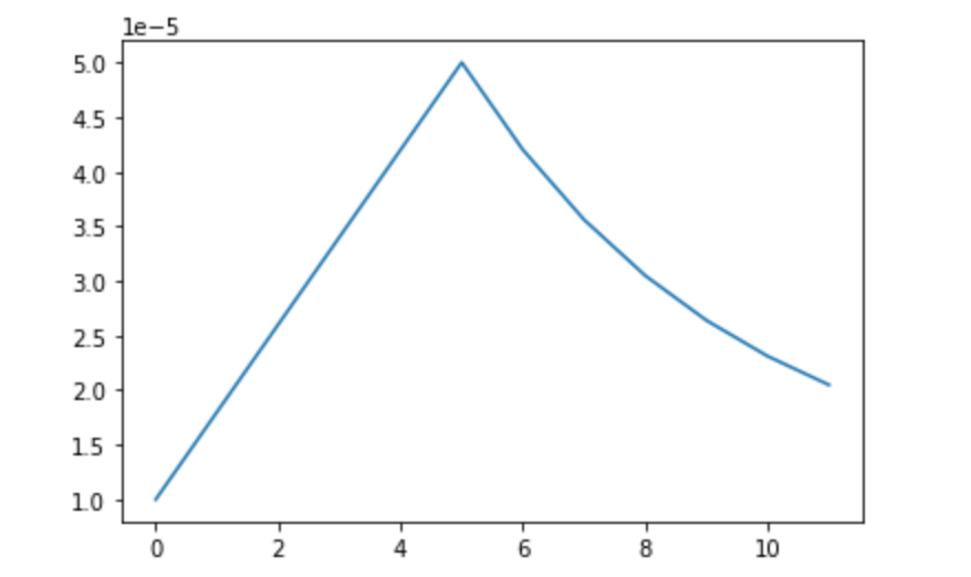
学习率计划
我们将使用特殊的学习率计划来训练该网络。
1 | # Learning Rate Schedule for Fine Tuning # |
结果输出为:
1 | Learning rate schedule: 1e-05 to 5e-05 to 2.05e-05 |
拟合模型
现在我们准备好训练模型了。定义了一些参数后,我们就可以开始了!
1 | # Define training epochs |
结果输出为:
1 | Epoch 00001: LearningRateScheduler reducing learning rate to 0.0010000000474974513. |
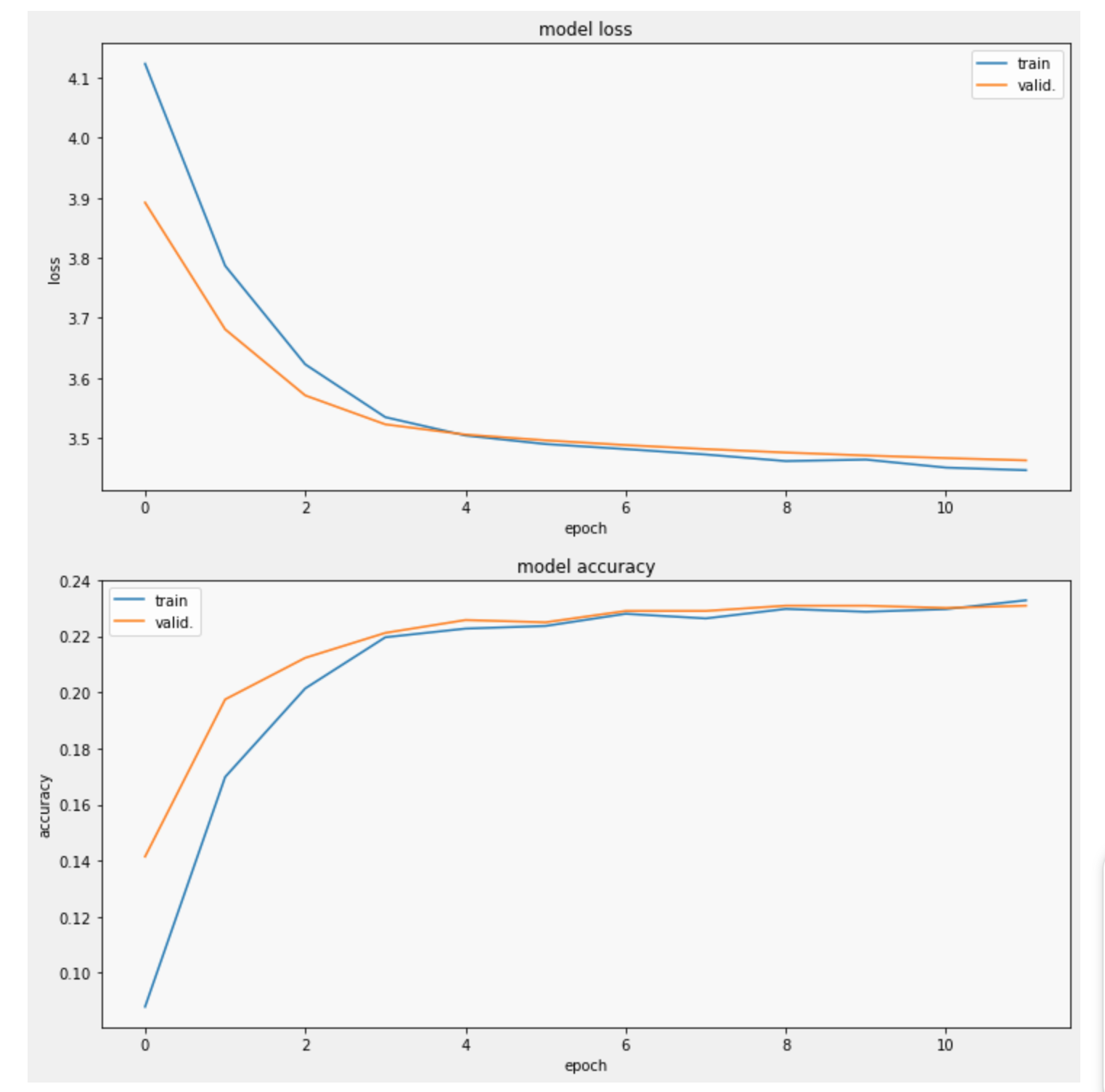
下一个单元格显示了训练期间损失和指标的进展情况。值得庆幸的是,它收敛了!
1 | display_training_curves( |
第7步:评估预测
在对测试集进行最终预测之前,最好在验证集上评估模型的预测。这可以帮助您诊断训练中的问题或建议改进模型的方法。我们将研究两种常见的验证方法:绘制混淆矩阵和视觉验证。
1 | import matplotlib.pyplot as plt |
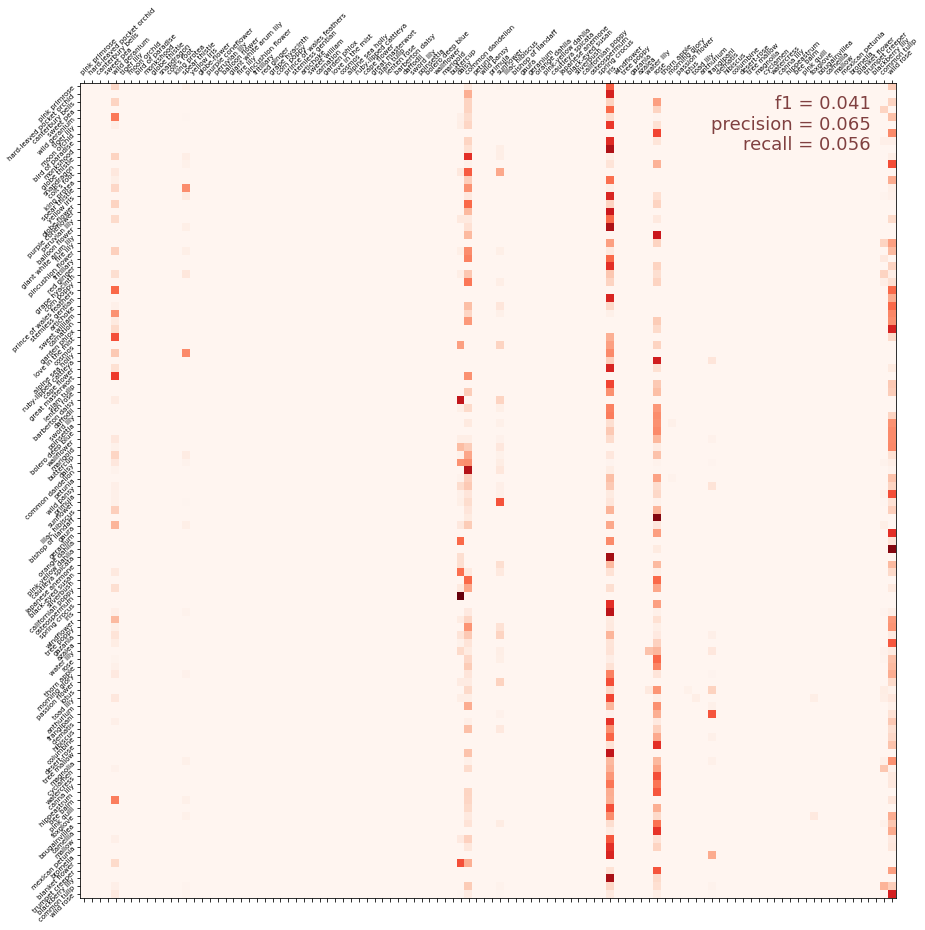
混淆矩阵
混淆矩阵显示了图像的实际类别与其预测类别的对比。它是评估分类器性能的最佳工具之一。以下单元格对验证数据进行一些处理,然后使用scikit-learn中包含的fusion_matrix函数创建矩阵。
1 | cmdataset = get_validation_dataset(ordered=True) |
您可能熟悉F1分数或精确率和召回率等指标。该单元格将计算这些指标并用混淆矩阵图显示它们。(这些指标在Scikit-learn模块sklearn.metrics中定义;我们已将它们导入到帮助程序脚本中。)
1 | score = f1_score( |
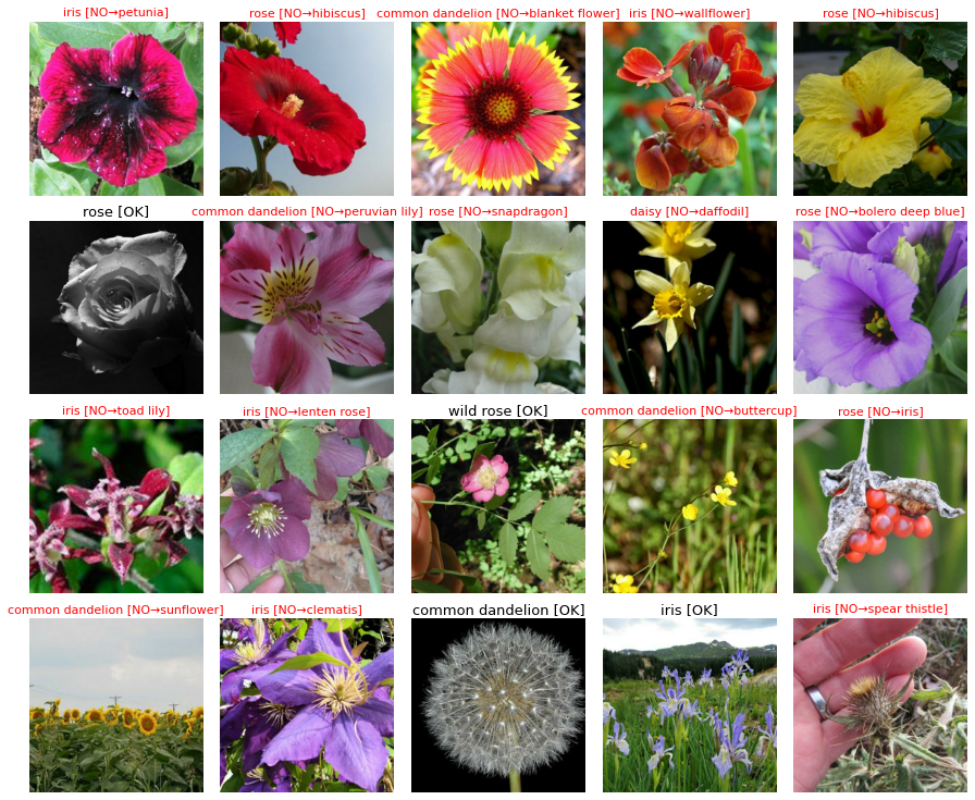
视觉验证
查看验证集中的一些示例并了解模型预测的类别也很有帮助。这可以帮助揭示模型遇到问题的图像类型的模式。此单元格会将验证集设置为一次显示20个图像 - 如果您愿意,您可以更改此设置以显示更多或更少图像。
1 | dataset = get_validation_dataset() |
这是一组花及其预测的种类。再次运行单元格以查看另一组。
1 | images, labels = next(batch) |
第8步:做出测试预测
一旦您对一切感到满意,您就可以对测试集进行预测了。
1 | test_ds = get_test_dataset(ordered=True) |
结果输出为:
1 | Computing predictions... |
我们将生成文件submission.csv。
1 | print('Generating submission.csv file...') |