特征工程实践之—房价预测

第1步 - 准备工作

导入和配置

我们将首先导入使用的包并设置一些笔记本默认值。

1
2
3
4
5
6
7
8
9
10
11
12
13
14
15
16
17
18
19
20
21
22
23
24
25
26
27
28
29
30
31
32
33
import os
import warnings
from pathlib import Path

import matplotlib.pyplot as plt
import numpy as np
import pandas as pd
import seaborn as sns
from IPython.display import display
from pandas.api.types import CategoricalDtype

from category_encoders import MEstimateEncoder
from sklearn.cluster import KMeans
from sklearn.decomposition import PCA
from sklearn.feature_selection import mutual_info_regression
from sklearn.model_selection import KFold, cross_val_score
from xgboost import XGBRegressor


# Set Matplotlib defaults
plt.style.use("seaborn-whitegrid")
plt.rc("figure", autolayout=True)
plt.rc(
"axes",
labelweight="bold",
labelsize="large",
titleweight="bold",
titlesize=14,
titlepad=10,
)

# Mute warnings
warnings.filterwarnings('ignore')
数据预处理

在进行任何特征工程之前,我们需要对数据进行预处理,以使其成为适合分析的形式。我们在课程中使用的数据比比赛数据简单一些。对于艾姆斯竞赛数据集,我们需要:

  • CSV文件加载数据。
  • 清理数据以修复任何错误或不一致。
  • 对统计数据类型(数字、分类)进行编码。
  • 估算任何缺失值。
加载数据

我们将把所有这些步骤包装在一个函数中,这将使您可以在需要时轻松获得新的数据帧。读取CSV文件后,我们将应用三个预处理步骤:清理、编码和插补,然后创建数据分割:一个 (df_train) 用于训练模型,另一个 (df_test) 用于进行预测。

1
2
3
4
5
6
7
8
9
10
11
12
13
14
15
def load_data():
# Read data
data_dir = Path("../input/house-prices-advanced-regression-techniques/")
df_train = pd.read_csv(data_dir / "train.csv", index_col="Id")
df_test = pd.read_csv(data_dir / "test.csv", index_col="Id")
# Merge the splits so we can process them together
df = pd.concat([df_train, df_test])
# Preprocessing
df = clean(df)
df = encode(df)
df = impute(df)
# Reform splits
df_train = df.loc[df_train.index, :]
df_test = df.loc[df_test.index, :]
return df_train, df_test
清理数据

该数据集中的一些分类特征在其类别中存在明显的拼写错误:

1
2
3
4
data_dir = Path("../input/house-prices-advanced-regression-techniques/")
df = pd.read_csv(data_dir / "train.csv", index_col="Id")

df.Exterior2nd.unique()

结果输出为:

1
2
3
array(['VinylSd', 'MetalSd', 'Wd Shng', 'HdBoard', 'Plywood', 'Wd Sdng',
'CmentBd', 'BrkFace', 'Stucco', 'AsbShng', 'Brk Cmn', 'ImStucc',
'AsphShn', 'Stone', 'Other', 'CBlock'], dtype=object)

将它们与data_description.txt进行比较可以向我们展示哪些内容需要清理。我们将在这里解决几个问题,但您可能需要进一步评估这些数据。

1
2
3
4
5
6
7
8
9
10
11
12
13
def clean(df):
df["Exterior2nd"] = df["Exterior2nd"].replace({"Brk Cmn": "BrkComm"})
# Some values of GarageYrBlt are corrupt, so we'll replace them
# with the year the house was built
df["GarageYrBlt"] = df["GarageYrBlt"].where(df.GarageYrBlt <= 2010, df.YearBuilt)
# Names beginning with numbers are awkward to work with
df.rename(columns={
"1stFlrSF": "FirstFlrSF",
"2ndFlrSF": "SecondFlrSF",
"3SsnPorch": "Threeseasonporch",
}, inplace=True,
)
return df
对统计数据类型进行编码

Pandas具有与标准统计类型(数值、分类等)相对应的Python类型。使用正确的类型对每个特征进行编码有助于确保我们使用的任何函数都适当地处理每个特征,并使我们更容易一致地应用转换。该隐藏单元定义了编码函数:

1
2
3
4
5
6
7
8
9
10
11
12
13
14
15
16
17
18
19
20
21
22
23
24
25
26
27
28
29
30
31
32
33
34
35
36
37
38
39
40
41
42
43
44
45
46
47
48
49
50
51
52
53
54
55
56
57
58
59
# The numeric features are already encoded correctly (`float` for
# continuous, `int` for discrete), but the categoricals we'll need to
# do ourselves. Note in particular, that the `MSSubClass` feature is
# read as an `int` type, but is actually a (nominative) categorical.

# The nominative (unordered) categorical features
features_nom = ["MSSubClass", "MSZoning", "Street", "Alley", "LandContour", "LotConfig", "Neighborhood", "Condition1", "Condition2", "BldgType", "HouseStyle", "RoofStyle", "RoofMatl", "Exterior1st", "Exterior2nd", "MasVnrType", "Foundation", "Heating", "CentralAir", "GarageType", "MiscFeature", "SaleType", "SaleCondition"]


# The ordinal (ordered) categorical features

# Pandas calls the categories "levels"
five_levels = ["Po", "Fa", "TA", "Gd", "Ex"]
ten_levels = list(range(10))

ordered_levels = {
"OverallQual": ten_levels,
"OverallCond": ten_levels,
"ExterQual": five_levels,
"ExterCond": five_levels,
"BsmtQual": five_levels,
"BsmtCond": five_levels,
"HeatingQC": five_levels,
"KitchenQual": five_levels,
"FireplaceQu": five_levels,
"GarageQual": five_levels,
"GarageCond": five_levels,
"PoolQC": five_levels,
"LotShape": ["Reg", "IR1", "IR2", "IR3"],
"LandSlope": ["Sev", "Mod", "Gtl"],
"BsmtExposure": ["No", "Mn", "Av", "Gd"],
"BsmtFinType1": ["Unf", "LwQ", "Rec", "BLQ", "ALQ", "GLQ"],
"BsmtFinType2": ["Unf", "LwQ", "Rec", "BLQ", "ALQ", "GLQ"],
"Functional": ["Sal", "Sev", "Maj1", "Maj2", "Mod", "Min2", "Min1", "Typ"],
"GarageFinish": ["Unf", "RFn", "Fin"],
"PavedDrive": ["N", "P", "Y"],
"Utilities": ["NoSeWa", "NoSewr", "AllPub"],
"CentralAir": ["N", "Y"],
"Electrical": ["Mix", "FuseP", "FuseF", "FuseA", "SBrkr"],
"Fence": ["MnWw", "GdWo", "MnPrv", "GdPrv"],
}

# Add a None level for missing values
ordered_levels = {key: ["None"] + value for key, value in
ordered_levels.items()}


def encode(df):
# Nominal categories
for name in features_nom:
df[name] = df[name].astype("category")
# Add a None category for missing values
if "None" not in df[name].cat.categories:
df[name] = df[name].cat.add_categories("None")
# Ordinal categories
for name, levels in ordered_levels.items():
df[name] = df[name].astype(CategoricalDtype(levels,
ordered=True))
return df
处理缺失值

现在处理缺失值将使特征工程进行得更加顺利。我们将缺失数值归为0,将缺失分类值归为“无”。您可能想尝试其他插补策略。特别是,您可以尝试创建“缺失值”指标:每当估算值时为1,否则为 0

1
2
3
4
5
6
def impute(df):
for name in df.select_dtypes("number"):
df[name] = df[name].fillna(0)
for name in df.select_dtypes("category"):
df[name] = df[name].fillna("None")
return df
加载数据

现在我们可以调用数据加载器并获取处理后的数据分割:

1
df_train, df_test = load_data()

如果您想查看它们包含的内容,请取消注释并运行此单元格。请注意,df_test缺少SalePrice值。(在插补步骤中NA被设为0。)

建立基线

最后,让我们建立一个基线分数来判断我们的特征工程。它将计算功能集的交叉验证RMSLE分数。我们的模型使用了XGBoost,但您可以想尝试其他模型。

1
2
3
4
5
6
7
8
9
10
11
12
13
14
15
16
def score_dataset(X, y, model=XGBRegressor()):
# Label encoding for categoricals
#
# Label encoding is good for XGBoost and RandomForest, but one-hot
# would be better for models like Lasso or Ridge. The `cat.codes`
# attribute holds the category levels.
for colname in X.select_dtypes(["category"]):
X[colname] = X[colname].cat.codes
# Metric for Housing competition is RMSLE (Root Mean Squared Log Error)
log_y = np.log(y)
score = cross_val_score(
model, X, log_y, cv=5, scoring="neg_mean_squared_error",
)
score = -1 * score.mean()
score = np.sqrt(score)
return score

当我们想要尝试新的特征集时,我们可以随时重用这个评分函数。我们现在将在没有附加功能的处理数据上运行它并获得基线分数:

1
2
3
4
5
X = df_train.copy()
y = X.pop("SalePrice")

baseline_score = score_dataset(X, y)
print(f"Baseline score: {baseline_score:.5f} RMSLE")

结果输出为:

1
Baseline score: 0.14302 RMSLE

这个基线分数可以帮助我们了解我们组装的某些特征是否实际上带来了任何改进。

第2步 - 特征有效分值

我们了解了如何使用互信息来计算某个特征的有效分值,让您了解该特征的潜力有多大。

1
2
3
4
5
6
7
8
9
10
11
12
13
14
15
16
17
18
19
def make_mi_scores(X, y):
X = X.copy()
for colname in X.select_dtypes(["object", "category"]):
X[colname], _ = X[colname].factorize()
# All discrete features should now have integer dtypes
discrete_features = [pd.api.types.is_integer_dtype(t) for t in X.dtypes]
mi_scores = mutual_info_regression(X, y, discrete_features=discrete_features, random_state=0)
mi_scores = pd.Series(mi_scores, name="MI Scores", index=X.columns)
mi_scores = mi_scores.sort_values(ascending=False)
return mi_scores


def plot_mi_scores(scores):
scores = scores.sort_values(ascending=True)
width = np.arange(len(scores))
ticks = list(scores.index)
plt.barh(width, scores)
plt.yticks(width, ticks)
plt.title("Mutual Information Scores")

让我们再次看看我们的特征得分:

1
2
3
4
5
X = df_train.copy()
y = X.pop("SalePrice")

mi_scores = make_mi_scores(X, y)
mi_scores

结果输出为:

1
2
3
4
5
6
7
8
9
10
11
12
OverallQual     0.571457
Neighborhood 0.526220
GrLivArea 0.430395
YearBuilt 0.407974
LotArea 0.394468
...
PoolQC 0.000000
MiscFeature 0.000000
MiscVal 0.000000
MoSold 0.000000
YrSold 0.000000
Name: MI Scores, Length: 79, dtype: float64

您可以看到,我们有许多信息丰富的特征,但也有一些特征似乎根本没有信息(至少其本身)。得分最高的特征通常会在特征开发过程中获得最大的回报,因此将精力集中在这些特征上可能是个好主意。 另一方面,对无信息特征的训练可能会导致过度拟合。因此,我们将完全放弃得分为0.0的特征:

1
2
def drop_uninformative(df, mi_scores):
return df.loc[:, mi_scores > 0.0]

删除它们确实会带来一定的性能提升:

1
2
3
4
5
X = df_train.copy()
y = X.pop("SalePrice")
X = drop_uninformative(X, mi_scores)

score_dataset(X, y)

结果输出为:

1
0.14274827027030276

稍后,我们会将drop_uninformative函数添加到我们的特征创建管道中。

第3步 - 创建特征

现在我们将开始开发我们的特征集。为了使我们的特征工程工作流程更加模块化,我们将定义一个函数,该函数将获取准备好的数据帧并将其通过转换管道传递以获得最终的特征集。它看起来像这样:

1
2
3
4
5
6
7
8
def create_features(df):
X = df.copy()
y = X.pop("SalePrice")
X = X.join(create_features_1(X))
X = X.join(create_features_2(X))
X = X.join(create_features_3(X))
# ...
return X

现在让我们继续定义一个转换,即分类特征的标签编码:

1
2
3
4
5
def label_encode(df):
X = df.copy()
for colname in X.select_dtypes(["category"]):
X[colname] = X[colname].cat.codes
return X

当您使用像XGBoost这样的树集成时,标签编码适用于任何类型的分类特征,即使对于无序类别也是如此。如果您想尝试线性回归模型,您可能会想使用one-hot编码,特别是对于具有无序类别的特征。

使用 Pandas 创建特征
1
2
3
4
5
6
7
8
9
10
11
12
13
14
15
16
17
18
19
20
21
22
23
24
25
26
27
28
29
30
31
32
33
34
35
36
37
38
39
def mathematical_transforms(df):
X = pd.DataFrame() # dataframe to hold new features
X["LivLotRatio"] = df.GrLivArea / df.LotArea
X["Spaciousness"] = (df.FirstFlrSF + df.SecondFlrSF) / df.TotRmsAbvGrd
# This feature ended up not helping performance
# X["TotalOutsideSF"] = \
# df.WoodDeckSF + df.OpenPorchSF + df.EnclosedPorch + \
# df.Threeseasonporch + df.ScreenPorch
return X


def interactions(df):
X = pd.get_dummies(df.BldgType, prefix="Bldg")
X = X.mul(df.GrLivArea, axis=0)
return X


def counts(df):
X = pd.DataFrame()
X["PorchTypes"] = df[[
"WoodDeckSF",
"OpenPorchSF",
"EnclosedPorch",
"Threeseasonporch",
"ScreenPorch",
]].gt(0.0).sum(axis=1)
return X


def break_down(df):
X = pd.DataFrame()
X["MSClass"] = df.MSSubClass.str.split("_", n=1, expand=True)[0]
return X


def group_transforms(df):
X = pd.DataFrame()
X["MedNhbdArea"] = df.groupby("Neighborhood")["GrLivArea"].transform("median")
return X

以下是您可以探索其他的一些想法:

  • 质量Qual和条件Cond特征之间的相互作用。例如,OverallQual就是一个高分特征。您可以尝试将其与OverallCond结合起来,方法是将两者都转换为整数类型并取一个乘积。
  • 面积特征的平方根。这会将平方英尺的单位转换为英尺。
  • 数字特征的对数。如果某个特征具有偏态分布,则应用对数可以帮助将其标准化。
  • 描述同一事物的数字特征和分类特征之间的相互作用。例如,您可以查看BsmtQualTotalBsmtSF之间的交互。
  • Neighborhood中的其他群体统计数据。我们做了GrLivArea的中位数。查看平均值、标准差或计数可能会很有趣。您还可以尝试将组统计数据与其他功能结合起来。也许GrLivArea和中位数的差异很重要?
k均值聚类

我们用来创建特征的第一个无监督算法是k均值聚类。我们看到,您可以使用聚类标签作为特征(包含 0、1、2、… 的列),也可以使用观测值到每个聚类的距离。我们看到这些特征有时如何有效地理清复杂的空间关系。

1
2
3
4
5
6
7
8
9
10
11
12
13
14
15
16
17
18
19
20
21
22
23
24
25
26
27
28
29
30
cluster_features = [
"LotArea",
"TotalBsmtSF",
"FirstFlrSF",
"SecondFlrSF",
"GrLivArea",
]


def cluster_labels(df, features, n_clusters=20):
X = df.copy()
X_scaled = X.loc[:, features]
X_scaled = (X_scaled - X_scaled.mean(axis=0)) / X_scaled.std(axis=0)
kmeans = KMeans(n_clusters=n_clusters, n_init=50, random_state=0)
X_new = pd.DataFrame()
X_new["Cluster"] = kmeans.fit_predict(X_scaled)
return X_new


def cluster_distance(df, features, n_clusters=20):
X = df.copy()
X_scaled = X.loc[:, features]
X_scaled = (X_scaled - X_scaled.mean(axis=0)) / X_scaled.std(axis=0)
kmeans = KMeans(n_clusters=20, n_init=50, random_state=0)
X_cd = kmeans.fit_transform(X_scaled)
# Label features and join to dataset
X_cd = pd.DataFrame(
X_cd, columns=[f"Centroid_{i}" for i in range(X_cd.shape[1])]
)
return X_cd
主成分分析

PCA是我们用于特征创建的第二个无监督模型。我们看到了如何使用它来分解数据中的变分结构。PCA算法为我们提供了描述变化的每个组成部分的载荷,以及转换后的数据点的组成部分。负载可以建议要创建的特征以及我们可以直接用作特征的成分。

1
2
3
4
5
6
7
8
9
10
11
12
13
14
15
16
17
18
19
20
21
22
23
24
25
26
27
28
29
30
31
32
33
34
35
36
37
38
39
def apply_pca(X, standardize=True):
# Standardize
if standardize:
X = (X - X.mean(axis=0)) / X.std(axis=0)
# Create principal components
pca = PCA()
X_pca = pca.fit_transform(X)
# Convert to dataframe
component_names = [f"PC{i+1}" for i in range(X_pca.shape[1])]
X_pca = pd.DataFrame(X_pca, columns=component_names)
# Create loadings
loadings = pd.DataFrame(
pca.components_.T, # transpose the matrix of loadings
columns=component_names, # so the columns are the principal components
index=X.columns, # and the rows are the original features
)
return pca, X_pca, loadings


def plot_variance(pca, width=8, dpi=100):
# Create figure
fig, axs = plt.subplots(1, 2)
n = pca.n_components_
grid = np.arange(1, n + 1)
# Explained variance
evr = pca.explained_variance_ratio_
axs[0].bar(grid, evr)
axs[0].set(
xlabel="Component", title="% Explained Variance", ylim=(0.0, 1.0)
)
# Cumulative Variance
cv = np.cumsum(evr)
axs[1].plot(np.r_[0, grid], np.r_[0, cv], "o-")
axs[1].set(
xlabel="Component", title="% Cumulative Variance", ylim=(0.0, 1.0)
)
# Set up figure
fig.set(figwidth=8, dpi=100)
return axs

其他特征变化

1
2
3
4
5
6
7
8
9
10
11
12
13
14
15
16
17
18
19
def pca_inspired(df):
X = pd.DataFrame()
X["Feature1"] = df.GrLivArea + df.TotalBsmtSF
X["Feature2"] = df.YearRemodAdd * df.TotalBsmtSF
return X


def pca_components(df, features):
X = df.loc[:, features]
_, X_pca, _ = apply_pca(X)
return X_pca


pca_features = [
"GarageArea",
"YearRemodAdd",
"TotalBsmtSF",
"GrLivArea",
]

这些只是使用主要成分的几种方法。您还可以尝试使用一个或多个成分进行组合。需要注意的一件事是,PCA不会改变点之间的距离——它就像旋转一样。因此,使用全套成分进行聚类与使用原始特征进行聚类相同。相反,选择成分的一些子集,可能是方差最大或MI分数最高的成分。为了进一步分析,您可能需要查看数据集的相关矩阵:

1
2
3
4
5
6
7
8
9
10
11
12
13
def corrplot(df, method="pearson", annot=True, **kwargs):
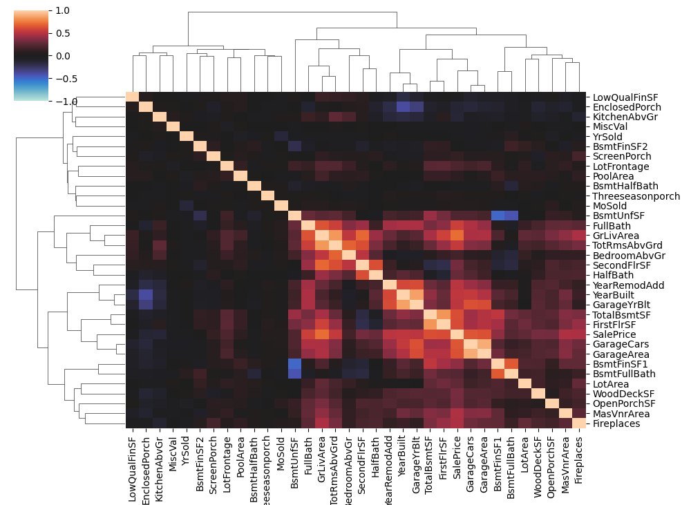
sns.clustermap(
df.corr(method, numeric_only=True),
vmin=-1.0,
vmax=1.0,
cmap="icefire",
method="complete",
annot=annot,
**kwargs,
)


corrplot(df_train, annot=None)

高度相关的特征组通常会产生有趣的负载。

PCA 应用 - 指示异常值

您应用了PCA来确定异常值的房屋,即房屋的值在其余数据中没有得到很好的体现。您看到爱德华兹附近有一组房屋的销售条件为“部分”,其价值特别极端。某些模型可以从指示这些异常值中受益,这就是下一个转换将要做的事情。

1
2
3
4
def indicate_outliers(df):
X_new = pd.DataFrame()
X_new["Outlier"] = (df.Neighborhood == "Edwards") & (df.SaleCondition == "Partial")
return X_new

您还可以考虑将scikit-learnsklearn.preprocessing模块中的某种强大的缩放器应用于外围值,尤其是GrLivArea中的值。这是一个说明其中一些的教程。另一种选择可能是使用 scikit-learn的异常值检测器之一创建“异常值分数”特征。

目标编码

需要单独的保留集来创建目标编码是相当浪费数据的。我们使用了25%的数据集来对单个特征(邮政编码)进行编码。我们根本没有使用那25%中其他特征的数据。然而,有一种方法可以使用目标编码,而不必使用保留的编码数据。 这基本上与交叉验证中使用的技巧相同:

  • 将数据拆分为折叠,每个折叠都有数据集的两个分割。
  • 在一个分割上训练编码器,但转换另一个分割的值。对所有分割重复此操作。

这样,训练和转换始终在独立的数据集上进行,就像使用保留集但不会浪费任何数据一样。 下面是一个包装器:

1
2
3
4
5
6
7
8
9
10
11
12
13
14
15
16
17
18
19
20
21
22
23
24
25
26
27
28
29
30
31
32
33
34
35
36
37
38
39
class CrossFoldEncoder:
def __init__(self, encoder, **kwargs):
self.encoder_ = encoder
self.kwargs_ = kwargs # keyword arguments for the encoder
self.cv_ = KFold(n_splits=5)

# Fit an encoder on one split and transform the feature on the
# other. Iterating over the splits in all folds gives a complete
# transformation. We also now have one trained encoder on each
# fold.
def fit_transform(self, X, y, cols):
self.fitted_encoders_ = []
self.cols_ = cols
X_encoded = []
for idx_encode, idx_train in self.cv_.split(X):
fitted_encoder = self.encoder_(cols=cols, **self.kwargs_)
fitted_encoder.fit(
X.iloc[idx_encode, :], y.iloc[idx_encode],
)
X_encoded.append(fitted_encoder.transform(X.iloc[idx_train, :])[cols])
self.fitted_encoders_.append(fitted_encoder)
X_encoded = pd.concat(X_encoded)
X_encoded.columns = [name + "_encoded" for name in X_encoded.columns]
return X_encoded

# To transform the test data, average the encodings learned from
# each fold.
def transform(self, X):
from functools import reduce

X_encoded_list = []
for fitted_encoder in self.fitted_encoders_:
X_encoded = fitted_encoder.transform(X)
X_encoded_list.append(X_encoded[self.cols_])
X_encoded = reduce(
lambda x, y: x.add(y, fill_value=0), X_encoded_list
) / len(X_encoded_list)
X_encoded.columns = [name + "_encoded" for name in X_encoded.columns]
return X_encoded

像这样:

1
2
encoder = CrossFoldEncoder(MEstimateEncoder, m=1)
X_encoded = encoder.fit_transform(X, y, cols=["MSSubClass"]))

您可以将category_encoders库中的任何编码器转换为交叉折叠编码器。CatBoostEncoder值得尝试。 它与MEstimateEncoder类似,但使用一些技巧来更好地防止过度拟合。其平滑参数称为a而不是m

创建最终的特征集

现在让我们将所有内容组合在一起。将转换放入单独的函数中可以更轻松地尝试各种组合。我发现那些未注释的结果给出了最好的结果。不过,您应该尝试自己的想法!修改任何这些转换或提出一些您自己的转换以添加到管道中。

1
2
3
4
5
6
7
8
9
10
11
12
13
14
15
16
17
18
19
20
21
22
23
24
25
26
27
28
29
30
31
32
33
34
35
36
37
38
39
40
41
42
43
44
45
46
47
48
49
50
51
52
53
54
55
56
57
58
def create_features(df, df_test=None):
X = df.copy()
y = X.pop("SalePrice")
mi_scores = make_mi_scores(X, y)

# Combine splits if test data is given
#
# If we're creating features for test set predictions, we should
# use all the data we have available. After creating our features,
# we'll recreate the splits.
if df_test is not None:
X_test = df_test.copy()
X_test.pop("SalePrice")
X = pd.concat([X, X_test])

# Lesson 2 - Mutual Information
X = drop_uninformative(X, mi_scores)

# Lesson 3 - Transformations
X = X.join(mathematical_transforms(X))
X = X.join(interactions(X))
X = X.join(counts(X))
# X = X.join(break_down(X))
X = X.join(group_transforms(X))

# Lesson 4 - Clustering
# X = X.join(cluster_labels(X, cluster_features, n_clusters=20))
# X = X.join(cluster_distance(X, cluster_features, n_clusters=20))

# Lesson 5 - PCA
X = X.join(pca_inspired(X))
# X = X.join(pca_components(X, pca_features))
# X = X.join(indicate_outliers(X))

X = label_encode(X)

# Reform splits
if df_test is not None:
X_test = X.loc[df_test.index, :]
X.drop(df_test.index, inplace=True)

# Lesson 6 - Target Encoder
encoder = CrossFoldEncoder(MEstimateEncoder, m=1)
X = X.join(encoder.fit_transform(X, y, cols=["MSSubClass"]))
if df_test is not None:
X_test = X_test.join(encoder.transform(X_test))

if df_test is not None:
return X, X_test
else:
return X


df_train, df_test = load_data()
X_train = create_features(df_train)
y_train = df_train.loc[:, "SalePrice"]

score_dataset(X_train, y_train)

结果输出为:

1
0.13863986787521657

第 4 步 - 超参数调整

在此阶段,您可能希望在创建最终提交之前使用XGBoost进行一些超参数调整:

1
2
3
4
5
6
7
8
9
10
11
12
13
14
15
16
17
X_train = create_features(df_train)
y_train = df_train.loc[:, "SalePrice"]

xgb_params = dict(
max_depth=6, # maximum depth of each tree - try 2 to 10
learning_rate=0.01, # effect of each tree - try 0.0001 to 0.1
n_estimators=1000, # number of trees (that is, boosting rounds) - try 1000 to 8000
min_child_weight=1, # minimum number of houses in a leaf - try 1 to 10
colsample_bytree=0.7, # fraction of features (columns) per tree - try 0.2 to 1.0
subsample=0.7, # fraction of instances (rows) per tree - try 0.2 to 1.0
reg_alpha=0.5, # L1 regularization (like LASSO) - try 0.0 to 10.0
reg_lambda=1.0, # L2 regularization (like Ridge) - try 0.0 to 10.0
num_parallel_tree=1, # set > 1 for boosted random forests
)

xgb = XGBRegressor(**xgb_params)
score_dataset(X_train, y_train, xgb)

结果输出为:

1
0.12417177287599078

只需手动调整这些即可给您带来很好的结果。但是,您可能想尝试使用scikit-learn的自动超参数调整器之一。或者您可以探索更高级的调优库,例如Optunascikit-optimize。以下是将OptunaXGBoost结合使用的方法:

1
2
3
4
5
6
7
8
9
10
11
12
13
14
15
16
17
18
19
import optuna

def objective(trial):
xgb_params = dict(
max_depth=trial.suggest_int("max_depth", 2, 10),
learning_rate=trial.suggest_float("learning_rate", 1e-4, 1e-1, log=True),
n_estimators=trial.suggest_int("n_estimators", 1000, 8000),
min_child_weight=trial.suggest_int("min_child_weight", 1, 10),
colsample_bytree=trial.suggest_float("colsample_bytree", 0.2, 1.0),
subsample=trial.suggest_float("subsample", 0.2, 1.0),
reg_alpha=trial.suggest_float("reg_alpha", 1e-4, 1e2, log=True),
reg_lambda=trial.suggest_float("reg_lambda", 1e-4, 1e2, log=True),
)
xgb = XGBRegressor(**xgb_params)
return score_dataset(X_train, y_train, xgb)

study = optuna.create_study(direction="minimize")
study.optimize(objective, n_trials=20)
xgb_params = study.best_params

第 5 步 - 训练模型并创建提交

一旦您对此感到满意,就可以创建最终预测了:

  • 从原始数据创建您的特征集
  • 在训练数据上训练
  • XGBoost使用经过训练的模型从测试集中进行预测
  • 将预测保存到CSV文件
1
2
3
4
5
6
7
8
9
10
11
12
X_train, X_test = create_features(df_train, df_test)
y_train = df_train.loc[:, "SalePrice"]

xgb = XGBRegressor(**xgb_params)
# XGB minimizes MSE, but competition loss is RMSLE
# So, we need to log-transform y to train and exp-transform the predictions
xgb.fit(X_train, np.log(y))
predictions = np.exp(xgb.predict(X_test))

output = pd.DataFrame({'Id': X_test.index, 'SalePrice': predictions})
output.to_csv('my_submission.csv', index=False)
print("Your submission was successfully saved!")