机器学习(中级)
介绍
- 处理现实世界数据集中常见的数据类型(缺失值、分类变量)。
- 设计管道以提高机器学习代码的质量。
- 使用先进的技术进行模型验证(交叉验证)。
- 构建最先进的模型,广泛用于赢得
Kaggle比赛(XGBoost)。 - 避免常见且重要的数据科学错误(泄漏)。
缺失值(Missing Values)
您将学习三种处理缺失值的方法。然后,您将在现实数据集上比较这些方法的有效性。
介绍
数据最终可能会出现缺失值的情况有很多。例如:
- 两居室的房子不包括第三间卧室的尺寸值。
- 调查受访者可以选择不分享他的收入。
如果您尝试使用缺失值的数据构建模型,大多数机器学习库(包括scikit-learn)都会出错。因此,您需要选择以下策略之一。
缺失值处理的三种方法
1.删除缺失值的列
最简单的选择是删除缺失值的列。
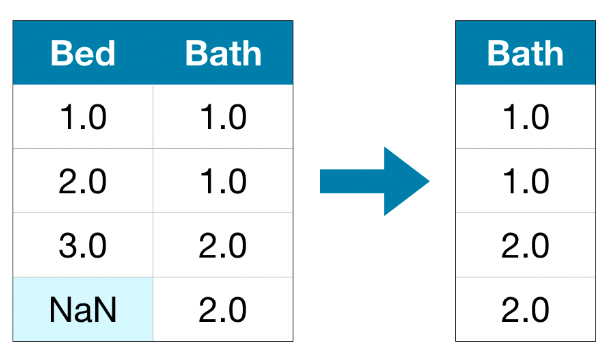
除非删除的列中的大多丢失数值,否则模型将无法使用此方法访问大量(可能有用!)信息。作为一个极端的示例,请考虑一个包含10,000行的数据集,其中一个重要列缺少单个条目。这种方法会完全删除该列!
2.更好的选择:插补
插补用一些数字填充缺失值。例如,我们可以填写每列的平均值。
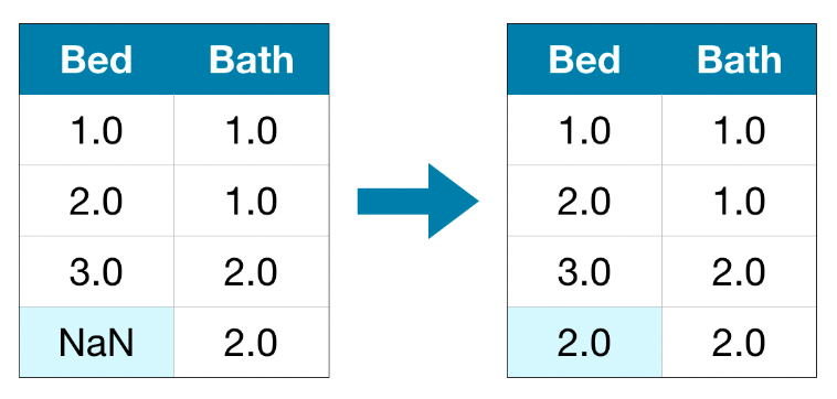
在大多数情况下,估算值并不完全正确,但与完全删除列相比,它通常会产生更准确的模型。
3.插补的扩展
插补是标准方法,通常效果很好。但是,估算值可能系统地高于或低于其实际值(未在数据集中收集)。或者,具有缺失值的行可能以其他方式是唯一的。在这种情况下,您的模型将通过考虑最初丢失的值来做出更好的预测。
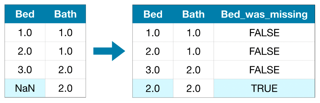
在这种方法中,我们像以前一样估算缺失值。此外,对于原始数据集中缺少条目的每一列,我们添加一个新列来显示估算条目的位置。就我而言,这将显着改善结果。在其他情况下,它根本没有帮助。
举例
在示例中,我们将使用墨尔本住房数据集。我们的模型将使用房间数量和土地面积等信息来预测房价。我们不会关注数据加载步骤。相反,您可以想象您已经在X_train、X_valid、y_train 和 y_valid中拥有训练和验证数据。
1 | import pandas as pd |
定义衡量每种方法质量的函数
我们定义一个函数Score_dataset()来比较处理缺失值的不同方法。此函数报告随机森林模型的平均绝对误差(MAE)。
1 | from sklearn.ensemble import RandomForestRegressor |
方法一的得分(删除具有缺失值的列)
由于我们同时使用训练集和验证集,因此我们会小心地在两个DataFrame中删除相同的列。
1 | # Get names of columns with missing values |
输出结果为:
1 | MAE from Approach 1 (Drop columns with missing values): |
方法二的得分(插补)
接下来,我们使用SimpleImputer将缺失值替换为每列的平均值。虽然很简单,但填充平均值通常效果很好(但这因数据集而异)。虽然统计学家尝试了更复杂的方法来确定估算值(例如回归估算),但一旦将结果插入复杂的机器学习模型,复杂的策略通常不会带来额外的好处。
1 | from sklearn.impute import SimpleImputer |
输出结果为:
1 | MAE from Approach 2 (Imputation): |
我们看到方法2的MAE低于方法1,因此方法2在此数据集上表现更好。
方法三的得分(插补的扩展)
接下来,我们估算缺失值,同时还跟踪估算了哪些值。
1 | # Make copy to avoid changing original data (when imputing) |
输出结果为:
1 | MAE from Approach 3 (An Extension to Imputation): |
正如我们所看到的,方法3的表现比方法2稍差。
那么,为什么插补比删除列表现更好呢?
训练数据有10864行和12列,其中3列包含缺失数据。对于每一列,缺失的条目不到一半。因此,删除列会删除很多有用的信息,因此插补会表现得更好是有道理的。
1 | # Shape of training data (num_rows, num_columns) |
1 | (10864, 12) |
结论
通常,相对于我们简单地删除包含缺失值的列(在方法1中),估算缺失值(在方法2和方法3中)会产生更好的结果。
分类变量(Categorical Variables)
介绍
分类变量仅采用有限数量的值。
- 考虑一项调查,询问您吃早餐的频率,并提供四个选项:“从不”、“很少”、“大多数天”或“每天”。在这种情况下,数据是分类的,因为响应属于一组固定的类别。
- 如果人们回答关于他们拥有什么品牌的汽车的调查,那么回答将分为“本田”、“丰田”和“福特”等类别。在这种情况下,数据也是分类的。
如果您尝试将这些变量插入到Python中的大多数机器学习模型中而不首先对其进行预处理,则会出现错误。我们将比较可用于准备分类数据的三种方法。
三种方法
删除分类变量
处理分类变量的最简单方法是将它们从数据集中删除。仅当列不包含有用信息时,此方法才有效。
序数编码
序数编码将每个唯一值分配给不同的整数。
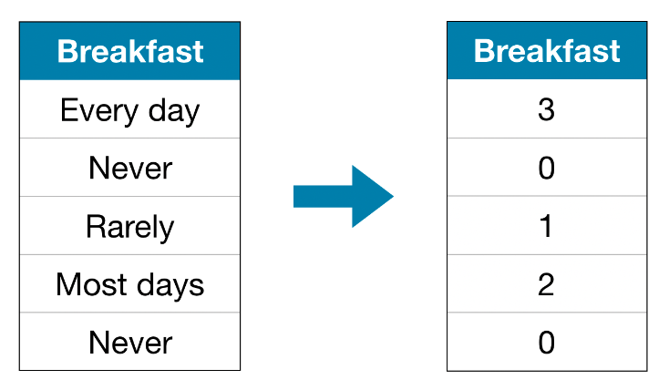
此方法假设类别的顺序为:“从不”(0)<“很少”(1)<“大多数天”(2)<“每天”(3)。这个假设在这个例子中是有意义的,因为类别有无可争议的排名。并非所有类别变量的值都有明确的排序,但我们将那些具有明确排序的变量称为序数变量。对于基于树的模型(例如决策树和随机森林),您可以期望序数编码能够很好地处理序数变量。
一次性编码
One-hot编码创建新列,指示原始数据中每个可能值的存在(或不存在)。为了理解这一点,我们将通过一个示例来进行操作。
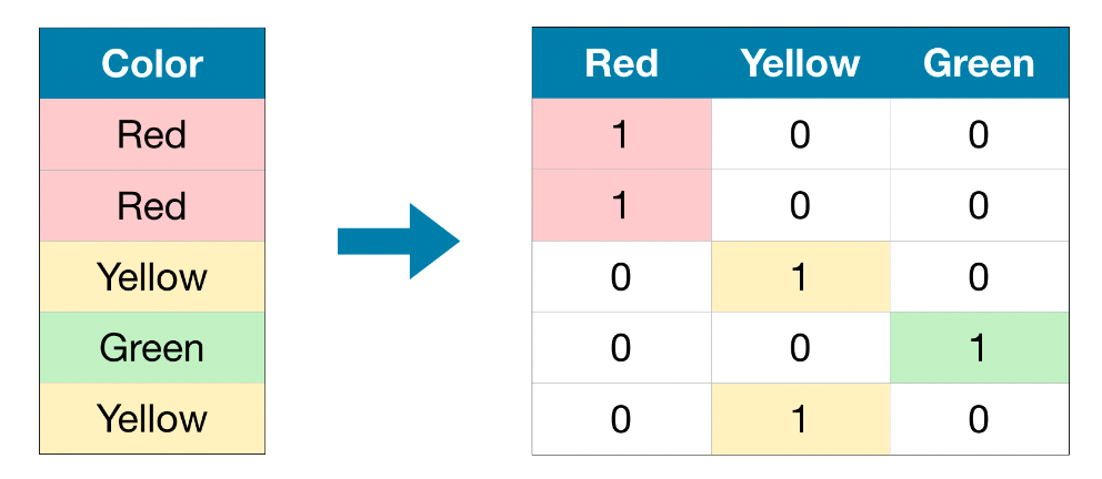
在原始数据集中,“颜色”是一个分类变量,具有三个类别:“红色”、“黄色”和“绿色”。相应的one-hot编码包含原始数据集中每个可能值的一列和每一行的一行。只要原始值为“Red”,我们就在“Red”列中输入1; 如果原始值为“黄色”,我们在“黄色”列中输入1,依此类推。与序数编码相反,one-hot编码不假设类别的顺序。因此,如果分类数据中没有明确的排序(例如,“红色”既不大于也不小于“黄色”),您可以预期这种方法会特别有效。我们将没有内在排名的分类变量称为名义变量。如果分类变量采用大量值(即,您通常不会将其用于采用超过15个不同值的变量),One-hot编码通常表现不佳。
举例
我们将使用墨尔本住房数据集。我们不会关注数据加载步骤。相反,您可以想象您已经在X_train、X_valid、y_train和y_valid中拥有训练和验证数据。
1 | import pandas as pd |
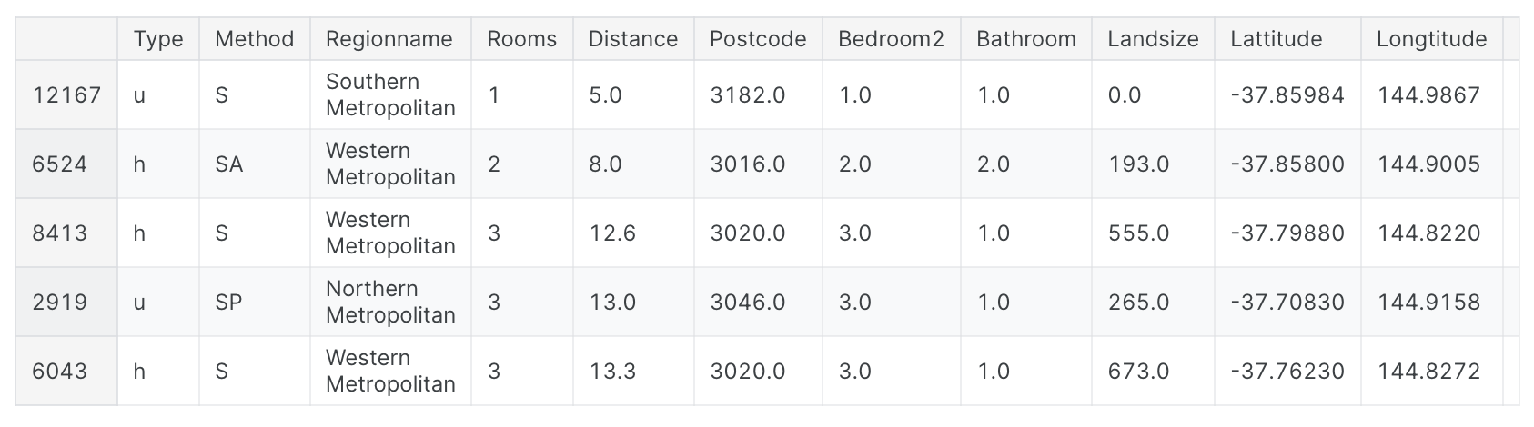
我们使用下面的head()方法查看训练数据。
1 | X_train.head() |
接下来,我们获得训练数据中所有分类变量的列表。我们通过检查每列的数据类型(或dtype)来做到这一点。对象数据类型指示列有文本(理论上它还可以是其他东西,但这对我们的目的来说并不重要)。对于此数据集,带有文本的列表示分类变量。
1 | # Get list of categorical variables |
结果输出为:
1 | Categorical variables: |
定义衡量每种方法质量的函数
我们定义一个函数Score_dataset()来比较处理calcategori变量的三种不同方法。此函数报告随机森林模型的平均绝对误差(MAE)。一般来说,我们希望MAE尽可能低!
1 | from sklearn.ensemble import RandomForestRegressor |
方法一的得分(删除类别变量)
我们使用select_dtypes()方法删除对象列。
1 | drop_X_train = X_train.select_dtypes(exclude=['object']) |
输出结果为:
1 | MAE from Approach 1 (Drop categorical variables): |
方法二的得分(序数编码)
Scikit-learn有一个OrdinalEncoder类,可用于获取序数编码。我们循环分类变量并将序数编码器分别应用于每一列。
1 | from sklearn.preprocessing import OrdinalEncoder |
输出结果为:
1 | MAE from Approach 2 (Ordinal Encoding): |
在上面的代码单元中,对于每一列,我们将每个唯一值随机分配给不同的整数,这是一种常见的方法,比提供自定义标签更简单;然而,如果我们为所有序数变量提供更明智的标签,我们可以期待性能的进一步提升。
方法三的得分(One-Hot 编码)
我们使用scikit-learn中的OneHotEncoder类来获取one-hot编码。有许多参数可用于自定义其行为。
- 我们设置
handle_unknown ='ignore'以避免当验证数据包含训练数据中未表示的类时出现错误。 - 设置稀疏
= False确保编码列作为numpy数组(而不是稀疏矩阵)返回。
为了使用编码器,我们只提供我们想要进行one-hot编码的分类列。例如,为了对训练数据进行编码,我们提供X_train[object_cols]。(下面代码单元中的object_cols是包含分类数据的列名称列表,因此X_train[object_cols]包含训练集中的所有分类数据。)
1 | from sklearn.preprocessing import OneHotEncoder |
输出结果为:
1 | MAE from Approach 3 (One-Hot Encoding): |
哪种方法最好?
在这种情况下,删除分类列(方法1)效果最差,因为它的MAE得分最高。至于其他两种方法,由于返回的MAE分数的值非常接近,因此其中一种方法似乎没有比另一种方法有任何有意义的好处。一般来说,one-hot编码(方法3)通常会表现最佳,而删除分类列(方法1)通常表现最差,但具体情况会有所不同。
总结
世界充满了分类数据。如果您知道如何使用这种常见数据类型,您将成为一名更高效的数据科学家!
管道
介绍
管道是保持数据预处理和建模代码井井有条的简单方法。具体来说,管道捆绑了预处理和建模步骤,因此您可以像使用单个步骤一样使用整个捆绑包。许多数据科学家在没有管道的情况下组合模型,但管道有一些重要的好处。其中包括:
- 更清晰的代码:在预处理的每个步骤中计算数据可能会变得混乱。使用管道,您无需在每个步骤中手动跟踪训练和验证数据。
- 错误更少:误用步骤或忘记预处理步骤的机会更少。
- 更容易生产:将模型从原型转变为可大规模部署的模型可能非常困难。我们不会在这里讨论许多相关的问题,但管道可以提供帮助。
- 模型验证的更多选项
举例
我们将使用墨尔本住房数据集。我们不会关注数据加载步骤。相反,您可以想象您已经在X_train、X_valid、y_train和y_valid中拥有训练和验证数据。
1 | import pandas as pd |
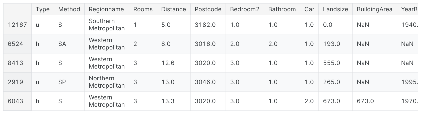
我们使用下面的head()方法查看训练数据。请注意,数据包含分类数据和具有缺失值的列。有了管道,就可以轻松处理这两件事!
1 | X_train.head() |
输出结果为:
我们分三步构建完整的管道。
第一步:定义预处理步骤
与管道如何将预处理和建模步骤捆绑在一起类似,我们使用ColumnTransformer类将不同的预处理步骤捆绑在一起。代码如下:
- 估算数值数据中的缺失值。
- 估算缺失值并对分类数据应用
one-hot编码。
1 | from sklearn.compose import ColumnTransformer |
第二步:定义模型
我们使用熟悉的RandomForestRegressor类定义随机森林模型
1 | from sklearn.ensemble import RandomForestRegressor |
第三步:创建并评估管道
最后,我们使用Pipeline类来定义捆绑预处理和建模步骤的管道。有一些重要的事情需要注意:
- 通过管道,我们预处理训练数据并在一行代码中拟合模型。(相反,如果没有管道,我们必须在单独的步骤中进行插补、
one-hot编码和模型训练。如果我们必须处理数值变量和分类变量,这会变得特别混乱!) - 通过管道,我们将
X_valid中未处理的特征提供给Predict()命令,管道在生成预测之前自动预处理这些特征。(但是,如果没有管道,我们必须记住在进行预测之前对验证数据进行预处理。)
1 | from sklearn.metrics import mean_absolute_error |
输出结果为:
1 | MAE: 160679.18917034855 |
结论
管道对于清理机器学习代码和避免错误非常有价值,对于具有复杂数据预处理的工作流程尤其有用。
交叉验证(Cross-Validation)
介绍
机器学习是一个迭代过程。您将面临有关使用哪些预测变量、使用什么类型的模型、为这些模型提供哪些参数等的选择。到目前为止,您已经通过验证来衡量模型质量,以数据驱动的方式做出了这些选择( 或坚持)设置。但这种方法有一些缺点。 要看到这一点,假设您有一个包含5000行的数据集。您通常会保留大约20%的数据作为验证数据集,即1000行。但这在确定模型分数时留下了一些随机机会。也就是说,模型可能在一组1000行上表现良好,即使它在不同的1000行上可能不准确。在极端情况下,您可以想象验证集中只有1行数据。如果您比较其他模型,哪个模型对单个数据点做出最好的预测将主要取决于运气!一般来说,验证集越大,我们衡量模型质量的随机性(也称为“噪声”)就越少,并且越可靠。不幸的是,我们只能通过从训练数据中删除行来获得大的验证集,而较小的训练数据集意味着更差的模型!
什么是交叉验证?
在交叉验证中,我们对不同的数据子集运行建模过程,以获得模型质量的多种度量。例如,我们可以首先将数据分为5部分,每部分占完整数据集的20%。在本例中,我们说我们已将数据分成5个“折叠”。
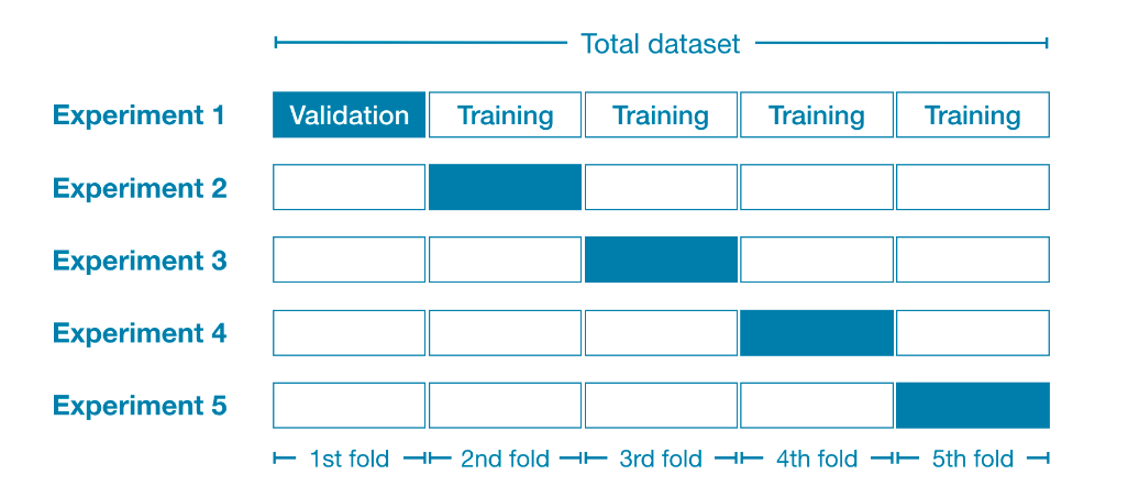
然后,我们为每个折叠运行一个实验:
- 在实验
1中,我们使用第一次折叠作为验证(或保留)集,其他所有内容作为训练数据。这为我们提供了基于20%保留集的模型质量衡量标准。 - 在实验
2中,我们保留第二次折叠中的数据(并使用除第二次折叠之外的所有数据来训练模型)。然后使用保留集来获得模型质量的第二次估计。 - 我们重复这个过程,使用每个折叠一次作为保留集。 总而言之。
100%的数据在某个时刻被用作保留,我们最终得到基于数据集中所有行的模型质量度量(即使我们不同时使用所有行)。
什么时候应该使用交叉验证?
交叉验证可以更准确地衡量模型质量,如果您要做出大量建模决策,这一点尤其重要。但是,它可能需要更长的时间来运行,因为它估计多个模型(每个折叠一个)。那么,考虑到这些权衡,您应该何时使用每种方法?
- 对于小型数据集,额外的计算负担并不是什么大问题,您应该运行交叉验证。
- 对于较大的数据集,单个验证集就足够了。您的代码将运行得更快,并且您可能拥有足够的数据,几乎不需要重复使用其中的一些数据来保留。
对于什么构成大数据集和小数据集,没有简单的阈值。但是,如果您的模型需要几分钟或更短的时间才能运行,则可能值得切换到交叉验证。或者,您可以运行交叉验证,看看每个实验的分数是否看起来很接近。如果每个实验产生相同的结果,则单个验证集可能就足够了。
举例
我们将使用与上一个教程中相同的数据。我们将输入数据加载到X中,将输出数据加载到y中。
1 | import pandas as pd |
然后,我们定义一个管道,使用输入器来填充缺失值,并使用随机森林模型来进行预测。虽然可以在没有管道的情况下进行交叉验证,但这非常困难!使用管道将使代码变得非常简单。
1 | from sklearn.ensemble import RandomForestRegressor |
我们使用scikit-learn中的cross_val_score()函数获取交叉验证分数。我们使用cv参数设置折叠次数。
1 | from sklearn.model_selection import cross_val_score |
结果输出为:
1 | MAE scores:[301628.7893587 303164.4782723 287298.331666 236061.84754543 260383.45111427] |
评分参数选择要报告的模型质量度量:在本例中,我们选择负平均绝对误差 (MAE)。scikit-learn的文档显示了选项列表。我们指定负MAE有点令人惊讶。Scikit-learn有一个约定,其中定义了所有指标,因此数字越大越好。在这里使用负数可以使它们与该约定保持一致,尽管负MAE在其他地方几乎闻所未闻。我们通常需要单一的模型质量度量来比较替代模型。所以我们取实验的平均值。
1 | print("Average MAE score (across experiments):") |
1 | Average MAE score (across experiments): |
结论
使用交叉验证可以更好地衡量模型质量,并具有清理代码的额外好处:请注意,我们不再需要跟踪单独的训练集和验证集。因此,特别是对于小型数据集,这是一个很好的改进!
XGBoost
您将学习如何使用梯度提升来构建和优化模型。该方法在许多Kaggle竞赛中占据主导地位,并在各种数据集上取得了成果。
介绍
您已经使用随机森林方法进行了预测,该方法通过对许多决策树的预测进行平均来实现比单个决策树更好的性能。我们将随机森林方法称为“集成方法”。根据定义,集成方法结合了多个模型的预测(例如,在随机森林的情况下是多个树)。接下来,我们将学习另一种称为梯度提升的集成方法。
梯度提升(Gradient boosting)
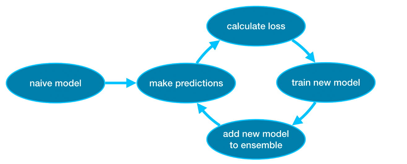
梯度提升是一种通过循环迭代将模型添加到集成中的方法。它首先使用单个模型初始化集成,该模型的预测可能非常幼稚。(即使它的预测非常不准确,随后对集合的添加也将解决这些错误。)然后,我们开始循环:
- 首先,我们使用当前的集合来为数据集中的每个观察生成预测。为了进行预测,我们将集合中所有模型的预测相加。
- 这些预测用于计算损失函数(例如均方误差)。
- 然后,我们使用损失函数来拟合将添加到集成中的新模型。具体来说,我们确定模型参数,以便将这个新模型添加到集成中将减少损失。(旁注:“梯度提升”中的“梯度”指的是我们将在损失函数上使用梯度下降来确定这个新模型中的参数。)。
- 最后,我们将新模型添加到集成中。
- 重复迭代。
![]()
举例
我们首先在 X_train、X_valid、y_train 和 y_valid 中加载训练和验证数据。
1 | import pandas as pd |
在此示例中,您将使用XGBoost库。XGBoost代表极限梯度提升,它是梯度提升的一种实现,具有一些注重性能和速度的附加功能。(Scikit-learn有另一个版本的梯度提升,但XGBoost有一些技术优势。)在下一个代码单元中,我们导入XGBoost的scikit-learn API(xgboost.XGBRegressor)。这使我们能够像在scikit-learn中一样构建和拟合模型。正如您将在输出中看到的,XGBRegressor类有许多可调参数——您很快就会了解这些!
1 | from xgboost import XGBRegressor |
结果输出为:
1 | XGBRegressor(base_score=0.5, booster='gbtree', callbacks=None, |
我们还进行预测并评估模型。
1 | from sklearn.metrics import mean_absolute_error |
输出结果为:
1 | Mean Absolute Error: 241041.5160392121 |
参数调整
XGBoost有一些参数可以显着影响准确性和训练速度。您应该了解的第一个参数是:n_estimators指定经历上述建模周期的次数。它等于我们包含在集成中的模型数量。
- 值太低会导致欠拟合,从而导致训练数据和测试数据的预测不准确。
- 太高的值会导致过拟合,从而导致对训练数据的预测准确,但对测试数据的预测不准确(这是我们关心的)。
典型值范围为100-1000,但这在很大程度上取决于下面讨论的learning_rate参数。以下是设置集成中模型数量的代码:
1 | my_model = XGBRegressor(n_estimators=500) |
输出结果为:
1 | XGBRegressor(base_score=0.5, booster='gbtree', callbacks=None, |
Early_stopping_rounds提供了一种自动查找n_estimators理想值的方法。当验证分数停止提高时,提前停止会导致模型停止迭代,即使我们没有处于n_estimators的硬停止状态。明智的做法是为n_estimators设置一个较高的值,然后使用Early_stopping_rounds来找到停止迭代的最佳时间。由于随机机会有时会导致单轮验证分数没有提高,因此您需要指定一个数字,表示在停止之前允许进行多少轮直接恶化。设置early_stopping_rounds=5是一个合理的选择。在这种情况下,我们在连续5轮验证分数恶化后停止。使用early_stopping_rounds时,您还需要留出一些数据来计算验证分数 - 这是通过设置eval_set参数来完成的。
我们可以修改上面的示例以包括提前停止:
1 | my_model = XGBRegressor(n_estimators=500) |
结果输出为:
1 | XGBRegressor(base_score=0.5, booster='gbtree', callbacks=None, |
如果您稍后想要使用所有数据来拟合模型,请将n_estimators设置为您在早期停止运行时发现的最佳值。我们不是通过简单地将每个组件模型的预测相加来获得预测,而是可以将每个模型的预测乘以一个小数(称为学习率),然后再添加它们。这意味着我们添加到集合中的每棵树对我们的帮助都会减少。因此,我们可以为n_estimators设置更高的值而不会过度拟合。如果我们使用提前停止,则会自动确定适当的树木数量。
一般来说,较小的学习率和大量的估计器将产生更准确的XGBoost模型,但模型的训练时间也会更长,因为它在循环中进行了更多的迭代。默认情况下,XGBoost设置learning_rate=0.1。修改上面的示例以更改学习率会产生以下代码:
1 | my_model = XGBRegressor(n_estimators=1000, learning_rate=0.05) |
结果输出为:
1 | XGBRegressor(base_score=0.5, booster='gbtree', callbacks=None, |
在考虑运行时间的较大数据集上,您可以使用并行性来更快地构建模型。通常将参数n_jobs设置为等于计算机上的核心数。对于较小的数据集,这没有帮助。生成的模型不会更好,因此对拟合时间进行微观优化通常只会分散注意力。但是,它在大型数据集中非常有用,否则您将在fit命令期间等待很长时间。这是修改后的示例:
1 | my_model = XGBRegressor(n_estimators=1000, learning_rate=0.05, n_jobs=4) |
结果输出为:
1 | XGBRegressor(base_score=0.5, booster='gbtree', callbacks=None, |
结论
XGBoost是一个领先的软件库,用于处理标准表格数据(存储在Pandas DataFrame中的数据类型,而不是图像和视频等更奇特的数据类型)。通过仔细调整参数,您可以训练高度准确的模型。
数据泄露(Data Leakage)
您将了解什么是数据泄漏以及如何防止数据泄漏。如果您不知道如何预防,泄漏就会频繁发生,并且会以微妙而危险的方式毁掉您的模型。因此,这是数据科学家实践中最重要的概念之一。
介绍
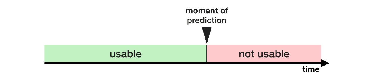
当你的训练数据包含有关目标的信息,但当模型用于预测时,类似的数据将不可用时,就会发生数据泄漏(或泄漏)。这会导致训练集(甚至可能是验证数据)上的高性能,但模型在生产中表现不佳。换句话说,泄漏会导致模型看起来很准确,直到您开始使用模型做出决策,然后模型就会变得非常不准确。泄漏主要有两种类型:目标泄漏和列车测试污染。
目标泄漏
当您的预测变量包含在您进行预测时不可用的数据时,就会发生目标泄漏。重要的是要根据数据可用的时间或时间顺序来考虑目标泄漏,而不仅仅是某个功能是否有助于做出良好的预测。一个例子会有所帮助。 想象一下,您想要预测谁会患上肺炎。原始数据的前几行如下所示:
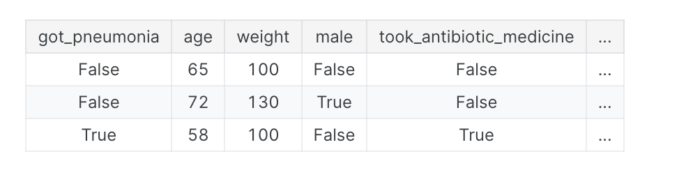
人们在患肺炎后服用抗生素药物才能康复。原始数据显示这些列之间存在很强的关系,但在确定got_pneumonia的值后,take_antibiotic_medicine经常发生更改。这就是目标泄漏。该模型会发现,任何take_antibiotic_medicine值为False的人都没有患有肺炎。由于验证数据与训练数据来自同一来源,因此该模式将在验证中重复,并且模型将具有很高的验证(或交叉验证)分数。但当随后在现实世界中部署时,该模型将非常不准确,因为当我们需要预测他们未来的健康状况时,即使是患有肺炎的患者也不会接受抗生素治疗。为了防止这种类型的数据泄漏,应排除在实现目标值后更新(或创建)的任何变量。
列车测试污染
当您不小心区分训练数据和验证数据时,就会发生另一种类型的泄漏。回想一下,验证旨在衡量模型如何处理之前未考虑过的数据。如果验证数据影响预处理行为,您可能会以微妙的方式破坏此过程。这有时称为列车测试污染。例如,假设您在调用train_test_split()之前运行预处理(例如为缺失值拟合输入器)。您的模型可能会获得良好的验证分数,让您对它充满信心,但在部署它来做出决策时却表现不佳。毕竟,您将验证或测试数据中的数据合并到预测中,因此即使无法推广到新数据,也可能在该特定数据上表现良好。当您进行更复杂的特征工程时,这个问题变得更加微妙(也更危险)。如果您的验证基于简单的训练测试分割,请从任何类型的拟合中排除验证数据,包括预处理步骤的拟合。如果您使用scikit-learn管道,这会更容易。使用交叉验证时,在管道内进行预处理更为重要!
举例
在本示例中,您将学习一种检测和消除目标泄漏的方法。我们将使用有关信用卡申请的数据集并跳过基本数据设置代码。最终结果是有关每个信用卡申请的信息都存储在DataFrame X中。我们将使用它来预测系列y中接受了哪些申请。
1 | import pandas as pd |
由于这是一个小数据集,我们将使用交叉验证来确保模型质量的准确测量。
1 | from sklearn.pipeline import make_pipeline |
结果输出为:
1 | Cross-validation accuracy: 0.981052 |
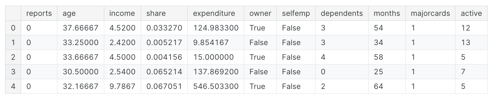
根据经验,您会发现很难找到准确率达到98%的模型。这种情况确实发生过,但这种情况并不常见,因此我们应该更仔细地检查数据是否存在目标泄漏。以下是数据摘要,您也可以在数据选项卡下找到:
card: 1 if credit card application accepted, 0 if notreports: Number of major derogatory reportsage: Age n years plus twelfths of a yearincome: Yearly income (divided by 10,000)share: Ratio of monthly credit card expenditure to yearly incomeexpenditure: Average monthly credit card expenditureowner: 1 if owns home, 0 if rentsselfempl: 1 if self-employed, 0 if notdependents: 1 + number of dependentsmonths: Months living at current addressmajorcards: Number of major credit cards heldactive: Number of active credit accounts
一些变量看起来很可疑。例如,支出是指这张卡上的支出还是申请前使用过的卡上的支出?此时,基本数据比较会非常有帮助:
1 | expenditures_cardholders = X.expenditure[y] |
结果输出为:
1 | Fraction of those who did not receive a card and had no expenditures: 1.00 |
如上所示,所有没有收到卡的人都没有支出,而只有2%的收到卡的人没有支出。我们的模型似乎具有很高的准确性,这并不奇怪。但这似乎也是一种目标泄漏的情况,其中支出可能意味着他们申请的卡上的支出。由于份额部分由支出决定,因此也应排除在外。 变量active和Majorcards不太清楚,但从描述来看,它们听起来令人担忧。在大多数情况下,如果您无法追踪创建数据的人以了解更多信息,那么安全总比后悔好。我们将运行一个没有目标泄漏的模型,如下所示:
1 | # Drop leaky predictors from dataset |
结果输出为:
1 | Cross-val accuracy: 0.830919 |
这个准确度相当低,这可能会令人失望。然而,我们可以预期,当在新应用程序中使用时,它的正确率约为80%,而泄漏模型的表现可能会比这差得多(尽管其在交叉验证中的明显得分更高)。
结论
在许多数据科学应用中,数据泄漏可能会造成数百万美元的错误。仔细分离训练和验证数据可以防止训练测试污染,而管道可以帮助实现这种分离。同样,谨慎、常识和数据探索的结合可以帮助识别目标泄漏。